After a very brief introduction to logic, I show how a type of path integral can be constructed in terms of propositional logic. This logic is then transformed into the Feynman Path Integral of quantum mechanics using general techniques.
Reality can be defined as the conjunction of all the facts we observe. Even space itself consists of a
collection of points all in conjunction with each other. And we describe each point
as having
individual coordinates. A conjunction of points, however, means that every point in fact logically implies every other point. And
it will be shown that an implication between two points equates to the disjunction of every possible
path from one point to another. Each path consists of a conjunction of implications, the first point
implying the second, in conjunction with the second point implying the third, in
conjunction with the third implying the forth, etc. Implication is then
represented in set theory using subsets, if a set exists, then its subset
exists. And the inclusion of a subset can be represented mathematically using
the Dirac measure, which equals 1 if the subset is included and is 0 otherwise.
This can be manipulated into the Kronecker delta,
ij,
which is 1 if i
j and is 0 if i
≠
j.
With implication represented by the Kronecker delta, it is
straightforward to show that disjunction is represented by addition, and that conjunction is represented by multiplication.
The disjunction of paths then has a
mathematical representation. In the case of a continuous space, the Kronecker
delta is replaced with the Dirac delta function. When the exponential Gaussian
function is used to represent the Dirac delta function, the
conjunction of implications for a path become the multiplication of exponential functions. The exponents then add up to form an Action integral, and the disjunction of every possible path forms the Feynman
Path Integral of quantum mechanics. This is 1st quantization. The wave function is the mathematical representation of logical implication. This process can be iterated to give us the quantum field theory of 2nd quantization. And the process can be iterated again to even give us 3rd quantization if needed. I also show where the Born Rule comes from to give us probabilities from the square modulus of the wave function. And finally, I give some reason to expect that these iterations prescribe that the complex numbers iterate to quaternions and
then to octonions, which are believed to be responsible for the U(1)×SU(2)×SU(3) symmetry of the Standard Model.
WEBSITE FEATURES:
There are a number of features programmed into this website to facilitate reading.
In the upper, left corner of the screen, there should appear a Section name to
tell you where you are in the document. You can use this to mark your place if
you should wish to continue reading at some other time.
Text
underlined with a gray line are tooltips. When you place the mouse over them,
additional text appears. Tooltips are used when reference is made to previous
equations. The equation itself appears in the tooltip so you don't have to
scroll back to them and loose your place.
You may resize the window or the text
without loosing your place. So you may shorten or lengthen the width of the
screen, or you may increase the size of the text to see more detail. To change
the size of the window, drag the edges of the window. To change the size of
the text, use Ctrl+mouse-wheel, or use the keyboard Ctrl+"+" or Ctrl+"-".
If a table or equation continues past the right edge of the screen, you
can either increase the size of the window, or you can decrease the size of
the text, or you can scroll to the right to see the rest of it. For normal
text just use the scroll bar to see the rest of it. For a tooltip, place the
cursor inside the tooltip and use Shift+mouse-wheel to scroll horizontally. Or
on the keyboard use Ctrl+right arrow, or Ctrl+left arrow.
For those not
that familiar with logic, I provide a means of checking the logic equations in
a truth-table generator. Cut and paste the equation into the generator to see
whether or not it is always true.
Finally, there is a comments
button at the bottom of the document to contact me with questions or comments.
Let me know if you find an error, or if you find something particularly
difficult.
Historically, quantum mechanics was developed in a rather ad-hoc manner, using trial and error to find some mathematics that eventually proved useful in making predictions. But the ultimate reasons why nature operates according to the equations of quantum mechanics has remained elusive. And some students of physics are mystified to the point of
frustrations by quantum mechanics because there does not seem to be any underlying principle
that justifies it. Where does the wave-function come from? How can the imaginary square-root of a probability have anything to do with reality? Some complain that it is counter-intuitive and even illogical. But the goal of this article is to prove that quantum mechanics can be derived from classical logic without any physical assumptions.
Those most interested in foundational issues are those exposed to the subject for the first time. It's usually easier to accept more complicated implications of a theory when the basic premises of it are well understood. Therefore, in order to broaden the audience, I include about a page worth of paragraphs briefly describing the basic introductory definitions in logic. And I include about a page worth of introduction to the integration process of calculus. The fundamentals in a subject should be relatively easy, so my intention is to keep this article under a sophomore college level. It is hoped that the ease of this material will be appreciated. The web pages I link to should contain a bibliography for those interested in further reading. Advanced readers can skip to the next section if they are familiar with the symbols used in logic.
Anyone can make claims about any subject they like, but that only brings up questions as to what evidence there is to support those claims and what those claims imply. And some may like to think they are being reasonable in what they believe. But how can we know that the conclusions they reach are correctly derived in a reasonable way? Logic is the study of correct argumentation. Given facts in relation to each other, logic is a tool to help us determine what other truths these facts equate to or imply. In this section I briefly touch on three topics in logic:
propositional logic, set theory, and predicate logic.
Propositional logic studies how the truth or falsity of statements effect the truth or falsity of other statements. Propositions are the same thing as statements or facts or claims which can either be true or they can be false, but they cannot be neither true nor false, and they cannot be both true and false at the same time. Propositional logic does not consider what the statements are about; it does not consider whether the statements are about abstract concepts such as math, or about physical facts or about feeling, emotions, or beauty. All
propositional logic does is label different statements with different letters such as a, b, c, etc.
and treats them as variables whose values can be either true or false. Then the
formulas of propositional logic can be applied to any subject and form the basis of valid reasoning about it. I will use T for true and F for False.
Compound statements can be constructed from simple statements using connectives such as AND and OR and IMPLIES and NOT. And the truth of the compound statement depends on how the simple statements are connected. Symbols are used for these connectives. I will use
for AND ( conjunction), for OR ( disjunction),and → for IMPLIES ( material implication),and
for NOT ( negation).
Below is a truth-table that shows the effect of these connectives on two statements, p and q.
1
2
3
4
5
p q
p
pq
pq
p → q
F F
T
F
F
T
F T
T
F
T
T
T F
F
F
T
F
T T
F
T
T
T
Column 1 in the table lists every possible combination of T and Fthat p and q can have. Column 2 shows that the operation of negation (NOT) has the effect of reversing the truth-valueof p.If p is T,then
p is F, and visa versa. Column 3 shows that the statement "p AND q"is T only when both p is Tand q is T.Column 4 shows that "p OR q"is T whenever either p is Tor q is T or when both are T. Material implication is the IF, THEN function of logic. If p implies q, this means if p is true,then q is true. To say that p implies q is the same thing as saying if p then q,or p proves q,or p therefore q,or p results in q,or p causes q, etc. Here the first operand, p, is called the premise, and the second operand, q, is called the consequence. Column 5 shows the relationship of material implication. It is true that p proves q for any truth-values of p and q except when p is Tbut q is F. The consequences might still be true regardless of the premises on which they're based, but you can not have premises that are true without consequences; that would mean there is not an implication between them. Some things to note are that conjunction (AND) is commutative, which means you can reverse the order of the operands, p and q, so you get p
qq
p. It is also true that disjunction (OR) is commutative. But implication (→) is not commutative, p → q is not equal to q → p.
You can find a more complete video lecture series on basic logic
here.
There is an on-line service that provides a
truth-table generator
here.
If you want to gain more confidence in these logic statements, simply enter
the statement in the box, and a truth-table will appear. However, text
characters must be entered for logic symbols. Use "/\" for AND,"\/" for OR,"=>" for IMPLIES,"~" for NOT, and "<=>" for EQUALS. For example, for the AND
statement enter the following text into the box (without the quotation marks):
"p/\q". For some of the logic expressions written below, a text version
is provided that you can cut and paste into this truth-table
generator.
Set theory constructs lists of objects called elements. For example, the set S whose elements are objects labeled aand band cand d is written as S{a,b,c,d}, where a
S symbolizes that a is an element of the set S. Then
set theory examines how differing sets can be combined. You can combine sets by considering the union of
sets, or the intersection between them or the complement of a set. For example, if you have only two sets, A {a,b,c,d,e,f} and B {d,e,f,g,h}, then the union between them is A
B{a,b,c,d,e,f,g,h}. The intersection of the two sets is A
B{d,e,f}. And if these two sets contain all the possible elements in the universe of our discourse, then the complement of B is
B{a,b,c}.It is also possible to have sets which are subsets of other sets. For example, the set C{a,c,e} is a subset of A, symbolized as C
A or as A
C which says
C is a subset of A, same thing as saying A is a superset of C.
Many times propositions can be described as objects with a particular property. In
predicate logic, if a specific object labeled q has the property labeled P,then Pq is the notation for saying it is true that q has the property P.The extension of a predicate, P,here labeled P, is the set of all those specific objects which have the property P.In other words,P{q1,q2,q3,q4}, where it is true that Pq1and Pq2and Pq3 and Pq4.The expansion of the predicate P is a proposition, here labeled P, which is the conjunction of statements of all those objects that have the property P.In symbols,PPq1Pq2Pq3Pq4.If it is understood that q1, q2, q3,and q4 are each propositions such that q1Pq1,q2Pq2,q3Pq3, and q4Pq4, then we can shorten the notation to P q1q2q3q4.And we can consider the consistency between all the statements in the set.
Consistency among statements in a theory means that no statement in the theory
can prove to be both true and false. And this means, of course, that no statement in the theory will prove itself false. So if we are given a set of statements that are asserted to be true, then consistency requires that no statement in the set will ever prove false any other statement in that set. Or in symbols,if q1 and q2 are asserted to coexist as true statements of the theory, then
Put ~(q1=> ~q2) <=>
(q1 /\ q2) in the
truth-table generator.
Notice that the result is true for all values of q1 and
q2. This means that it
is a valid argument in all circumstances. It is sometimes called a tautology.
And if Equation [2] is true between any two statements in the set, then a consistent set can be seen as the conjunction of all its statements:
q1q2q3...qnqi[3]
where all the qi belong to the same set, and where n could be infinite, and where the
symbol used here is the logical conjunction of n statements.
To apply these ideas to nature, we can say that reality consists of all the objects within it. We can use the letter U to symbolize the property of belonging to the universe, and symbols such as q1, q2,q3, q4, etc. to represent various kinds of objects. We write Uq1,Uq2,Uq3, etc. to represent the statements that those objects have the property of actually existing in the universe.We can abbreviate those statements as q1, q2, q3, etc., which means q1Uq1,q2Uq2,q3Uq3, etc., and they describe facts in the universe in terms of propositions that can be considered either true or false. The extension of the property U would be the set U{q1, q2, q3,...}, and the expansion of U would be the proposition Uq1q2q3...And we would say that the universe consists of all the facts in reality coexisting in conjunction with each other.
It may be that some of the facts, qi, might be broken down into a conjunction of even more propositions which represent even smaller objects that have differing properties. And it may be that still other facts, qj, may share some of these differing properties in common. But it's still clear that the extension of these differing properties are subsets of the universal set, U.And the expansion of these properties only contribute propositions that exist in conjunction with everything else. So we can ultimately describe the universe as consisting of a conjunction of all the facts that describe all the parts of the universe. We use propositions to describe individual facts in reality all the time. For we describe situations in nature with propositions - this physical situation has this or that property, it's made of these parts, it's located at this place at this time. And we often argue about whether a statement about reality is actually true.We use
the word "true" for those propositions that do describe what's real and "false"
for those propositions that do not describe what's real. Larger physical systems
are described with smaller physical subsystems. And we strive to find the
smallest constituents of reality which will themselves always end up being
described with one statement or another that we call true.
So nature can be considered to be a consistent set of statements. And we expect that no fact in reality will ever contradict any other fact in reality. Just looking around we see that the chair we are sitting on exists AND the floor holding up the chair exists AND the computer screen we are reading exists AND the room we are in exists AND the walls exist AND the doors of the room exist AND the atoms they are made of exist, etc, etc,ad infinitum. We presume this coexistence between facts at every level of existence down to the most microscopic level even though it is not observable with our eyes. For if this much were not true, I don't suppose we would be able to describe anything in reality. So in the most general sense, I think it's fair to describe reality at the smallest level as consisting of a consistent set of propositions. That isn't to say we know what all the facts are or what properties they have, but whatever laws of physics there are,
we suppose they come from some sort of underlying consistency.
Continuing from
Equation [3]
q1q2q3...qnqi
,
it should be realized that
q1q2→(q1→ q2)(q2→q1)[4]
Put (q1
/\ q2)
=> ((q1 =>
q2)
/\ (q2 =>
q1)) in the
truth-table generator. Notice that it is always true.
So what this means for the whole conjunction of reality is
qi→
(qi→
qj)
(qi→
qj)
[5]
This conjunction would include factors such as (qi→qi) which are true by the definition of material implication. And such factors do not change the conjunction since ppTfor any proposition p. You can always factor in a truth in a conjunction.
For example, if both i and j run from 1 to 4
in Equation [5], then the following conjunction is obtained, and you can put the following
equation in the
truth-table generator:
Notice that it is always true.
Also, notice that parenthesis are inserted between conjunctions to show which
conjunction is evaluated first. This does not interfere with the calculation
since abcd
a(b(cd
)).
The conjunction on the left hand side (LHS) of
Equation [5],
qi→
(qi→
qj)
only implies the right hand side (RHS); it is not an equivalence. When all the qi are T, the LHS equals the RHS, and both sides are T.If there is a mixture of T and F for the qi, then the LHSwill be F since there is an F in a conjunction.
But on the RHS, there will be factors of the form (F →T) T,
and when those same factors are reversed elsewhere in the conjunction, there will be factors of the form (T → F) F, making the conjunction on the RHS false just as it
is on the LHS. The only difference between the LHS and the RHS is when all the qi are F. Though the conjunction on the LHS is false when all qi are false, all the implications on the RHSare T when all the qi are F. This is because (F → F) T is a true statement by definition of implication.
Yet, if it is safe to at least assume that something in the set is true, then
Equation [5] becomes an effective equality. For then there will be an implication somewhere on the RHS of the form (T → F) F, which would make the conjunction on the RHS false just as the LHS would be. And in the case of reality, it's probably safe to assume that there must be something that truly exists. For we can at least say that the universe exists.
(Try changing the first => to the equal sign, <=>, for the last
equation inserted in the generator.)
So how are paths constructed? Consider the following:
((q0→q1)
((q0→q0)(q0→q1))
((q0→q1)(q1→q1)) ,
where q0 is the start of the path, and q1 is the
end of the path. This is obvious, because both
(q0→q0)
and (q1→q1)
are true, and we have qT
q. So we are left with (q0→q1)
(q0→q1),
but this is just (q0→q1)
since qq
q.
This can also be written as, (q0→q1) (q0→
qj)(qj→q1), where
is the disjunction of two terms.
Here I'm comparing an implication from q0 to q1 to a step in a path, for in some sense the premise leads us to the conclusion like a step from one place to another. The last equation represents a very short, one step path from q0 to q1, but we can insert intermediate steps. Let the start of the path be q0, and the end of the path be q2. And now let's insert an intermediate step, q1, between them. This is now a two step path, and the paths from q0 to q2
would give us,
There's no value of qj, T or F,
that can negate the equality of
Equation [6].
(q0→qn)
(q0→
qj)(qj→qn)
To prove this, there are two cases to consider: either
case 1:
(q0→qn)
F ,
or case 2: (q0→qn)
T.
In case 1
(q0→qn)
(q0→
qj)(qj→qn)
becomes
(T→F )
(T→
qj)(qj→F )
,
(q0→qn)
F, this can only happen if q0
T
and qn
F.
Then for
(q0→qn)
(q0→
qj)(qj→qn)
becomes
(T→F )
(T→
qj)(qj→F )
(T→F )
...
(T→
T)(T→F )
for
qj= T
a qj T, (q0→qj)
will be equal to (T →T), which is true. However, (qj→qn)
will be (T→F), which is false. And TFF. So that term in the disjunction
will be false.
But for
(q0→qn)
(q0→
qj)(qj→qn)
becomes
(T→F )
(T→
qj)(qj→F )
(T→F )
...
(T→
F)(F→F )
for
qj= T
a qj
F, (q0→qj)
will be equal to (T→F), which is false. So again that term in the
disjunction will be false.
So if
(q0→qn)
F, then all the terms will be false no matter the value of
qj, and both sides of
Equation [6]
(q0→qn)
(q0→
qj)(qj→qn)
will be false.
In case 2, (q0→qn)
T, this can happen in three ways. Way 1: q0
F
and
qn
T,
Way 2: q0
F
and
qn
F,
Way 3: q0
T
and
qn
T.
For Way 1,
(q0→qn)
(q0→
qj)(qj→qn)
will becomes
(F→T )
(F→
qj)(qj→T )
, for
q0 =
F and qn =
T
(F→T )
...
(F→
T)(T→T )
for
qj= T
(F→T )
...
(F→
F)(F→T )
for
qj= F
(q0→qj)
will be
(F→qj),
which is true for any
qj. And (qj→qn) will be (qj→
T), which is also true for any
qj. So all the disjunction terms will be true as
well. So both sides of
Equation [6]
(q0→qn)
(q0→
qj)(qj→qn)
will be true.
For Way 2
(q0→qn)
(q0→
qj)(qj→qn)
will becomes
(F→F )
(F→
qj)(qj→F )
, for
q0 =
F and qn =
F
(F→F )
...
(F→q0)(q0→F )
for
qj=q0
(F→F )
...
(F→
F )(F→F )
for
q0= F
, there will be at least one term that is true, namely, when
j0. For q0 has already been assigned to be false.
Then
(q0→qj) will be
(q0→q0), which is true, and
(qj→qn)
will be (q0→qn)(F→qn),
which is also true. This will make the
j0 term true, which makes the whole disjunction true.
For Way 3
(q0→qn)
(q0→
qj)(qj→qn)
will becomes
(T→T )
(T→
qj)(qj→T )
, for
q0 =
T and qn =
T
(T→T )
...
(T→qn)(qn→T )
for
qj=qn
(T→T )
...
(T→
T )(T→T )
for
qn= T
,
there will be at least one term that is true, namely, when
jn. For qn has already been assigned to be
true.
Then
(q0→qj) will be
(q0→qn)(qj→
T), which is true, and (qj→qn)
will be (qn→qn), which is also true. This will
make the
j=n term true, which makes the whole disjunction true.
So there is no value of
qj
that can
make the equality in
Equation [6]
(q0→qn)
(q0→
qj)(qj→qn)
a false statement.
Equation [6] represents n parallel paths of two steps each. The index j cycles through all n propositions in the universal set so that qj acts like a variable taking
the place of various
propositions. For each value of j, qj represents a different proposition. Note that since qj is the only variable in
Equation [6]. The factors (q0qj)
and (qjqn)
can be thought of as functions of the single variable qj, with q0 and qn
being held constant. Then Equation [6] can be thought of as a type of
mathematical expansion in terms of other functions.
Equation [6]
(q0→qn)
(q0→
qj)(qj→qn)
can be iterated to give all possible paths of 3
steps each. For example, let (q0→
qj) in Equation
[6] be,
(q0→qj)
(q0→
qi)(qi→qj).
And insert this into Equation [6] to get,
(q0→qn)
[
(q0→
qi)(qi→qj)](qj→qn),
which can be written as,
(q0→qn)
(q0→
qi)(qi→qj)(qj→qn).
And we can iterate this m number of times to get,
[7]
(q0→qn)
(q0→
q)(q→q)(q→q)(q→q)...(q→qn).
Each term in this disjunction is a path of m steps.
But this also includes terms like,
(q0→
q0)(q0→q0)(q0→q0)(q0→q0)...(q0→qn)
(q0→qn),
which is a 1 step path. So Equation [7] contains every possible path, including
paths of 1 step, 2 steps, 3 steps, up to m steps each.
If you want to check Equation
[7], the page here gives the logical
expression for Equation [7] when n=4 and m=3.
You may cut and paste this into the
truth-table generator. And you may
experiment with changing m.
are functions of two variables, since both q
and q act like variables which cycle through various propositions. If mn, so that the i's range through every possible state in the universal set, then Equation [7] is the combination of every possible path through the universal set. Already we can see this is setting us up to derive Feynman's
Path Integral.
All we need to do is find a means to map these logical operation to
mathematical operations. The next section is an effort to do just that.
could have been anticipated long ago. For it seems to represent every disagreement we have. We might agree about the state of affairs at some point in the past, and we might agree about some other point after that. But we might disagree about what sequence of events got us from the first point to the second point. One party proposes one sequence of event. The other party proposes a different sequence of events. And we are left considering the alternative sequences of events. For example, a man on trial for murder,
both parties agree that the victim was alive at some point and then was found dead at another point. Prosecution will argue that a series of events happened to prove that the accused committed the crime. Whereas, the Defense will argue a different sequence of events in which the man is innocent. The jury ends up considering alternative sequences of events.
Propositional logic uses connectives like AND and OR and NOT that operate on statements
that are true or false. But physics is expressed in terms of mathematical operations that
act on
numerical values. So if we wish to go from logic to math, we need a way to
assign mathematical operations to logical connectives and to give numerical
value to propositional statements.
It seems that mathematics itself is built on the foundation of set theory;
Zermelo–Fraenkel
set theory serves as the most common foundation of mathematics. And since we
are trying to find a mathematical expression for
that relies heavily on implication, we must ask if there is a set-theoretic representation of implication. It turns out that there is.
Implication is expressed in set theory using
subsets as shown
here. If a set exists, then any of its subsets exist. If the set A is
defined to be {a,b,c,d,e,f}, and set B is defined to be {c,d,e}, then if A
exists, B exists. This can be written as AB, which means A is a
superset of B. It is the same as writing BA,
which means B is a subset of A. This has the same truth-table as the material
implication of propositional logic. If A exists, then B exists. But if B
exists (or is defined), this does not mean that A exists. And if A does not
exist, then B cannot exist. What you cannot have is that A exists but B does
not; that would deny the definition of a subset. So we have a set-theoretical
definition of implication. But is there a numeric function for this set theory
implication?
Recall that a proposition, q,
can be written as Pq, which is true if the object q has the
property P and is false if q does not have the property
P.
But the property P has the extension P{q1,q2,q3,...}, the
set of all such objects that have that property. This
means that q is true if (q
P) and q is false if (q
P). So we have propositions and implications in terms of set theory. But
how does this relate to numbers?
Numbers are defined as the count of how many
elements are in a set; this is called the cardinality of a set. Zero is defined as the empty set, one is defined as the
set with one element, and two is defined as the set with two elements in it,
etc. If P is the extension of a property to which only q may belong, then
(q
P) mean that P is empty and has the cardinality of zero, and (q
P) means that P has the cardinality of one. So we seek a function with gives 1
for set inclusion and 0 otherwise.
The Dirac measure accomplishes this,
as shown here. The Dirac measure is denoted x(A) and is defined such that,
x(A)
1 if x
A
0 if x
A
where x is a possible element of some arbitrary set, A.
In the language here, if the proposition x (x
A) is true, then the Dirac measure maps x to the value of 1. And if
x is a false proposition
(or x
A), then the Dirac measure maps x to the value of 0. So the Dirac measure
maps T to 1and F to 0.
And this makes intuitive sense. For if we ask if whether some thing exists, then
if the answer is "yes, that's true", we have at least 1 sample of that thing.
But if the answer is "no, that's false", then we have zero samples of that
thing.
But if the set A has been defined to be the set {a,b,c,d,x,e,f,g,h}, then we can take the expansion of it to get
the proposition, A a^b^c^d^x^e^f ^g^h, where a (a A),b (b A), etc. And we can consider the truth and falsity of
the propositions Aand x independently from one another and ask how the truth-value of each are related.
IfAis true, then
so is x. But if A is false, this does not mean that
x
is false. It may be that any of a, b,
c, d, e,
f, g, or h
is false, which means the proposition A may include a conjunction with the statement, g, but the set A does
not include the element, g. However, if x is false, then so must A be false. We cannot have that x is false and A is true. This mimics the truth-table of implication.
Thus so far, we found that the inclusion or not of a subset within a set expresses logical implication. And we found that the Dirac measure gives a numeric value depending on whether a specific element is included or not in a set. We can recognize, however, that an element can be seen as a set of that single element. For it's always true that
(x {x}). Then the Dirac measure is a numeric representation of set inclusion, which is a set-theoretic representation of material implication. So we have a numeric function from logic to math.
But the situation we have is that all the propositions in
each describe the inclusion
or not of a corresponding element in a universal set. In other words, all the
proposition in Equation [7] represent elements, none are described as sets that contain
other elements. So the question is how do we use the Dirac measure to
represent implication between elements?
In the notation for the Daric measure, x(A), notice that x is an element and A is a set and not an element. Yet, we need
a math representation for the implication between one element and another element. For paths were constructed
in Equation [7] using the implication between propositions, where each proposition
describes a single element in the universal set. So we need to manipulate
x(A) to be more of the form x({y}), which would mathematically represent more closely the implication between two propositions.
To accomplish this, note that the set A in the notation of x(A)
is a set whose number of elements is not specified. So we should still have x(A) representing implication even if A is shrunk down to the size of an element. Let A shrink down to an element, call it y. Then,
in that case, we have A{y},
and we can write,
x(A)
x({y})
yx
1 if x y,
0 if x
≠
y.
For we know that if the element x is the element y, or xy, then x{y} would equal x{x}, which is inherently true
and gets mapped to 1. Otherwise,
if x ≠ y, then
x{x},where {x} is every element other than x. And we know that x{x} is an inherently false statement that gets mapped to 0.
Previously when we considered A{a,b,c,d,x,e,f,g,h}, the expansion was A a^b^c^d^x^e^f ^g^h. But now, when we think of A{y}, the expansion is A y. So A → x becomes y
→ x, and
x({y}) is a mathematical representation of y
→ x,
where x and y each refer to an element, which is what is needed for the conjunction of implications in Equation [7].
And it's appropriate that implication should be mapped to a function with numeric
valued, namely x({y}).
For the implication, y
→ x,
is also a statement in an of itself that evaluates to T
or F, depending on whether x or
y is T or F. So
its representation, x({y}),
should be 1 or 0 depending on whether x and
y maps to 1 or 0.
that the consequence in one implication is the premise in the next implication. And if we let x (x
{x}), for each x, then the proposition, x, can now represent either the element or the set.
So x can either be a premise or conclusion, whatever the implications require
in Equation [7].
I labeled x(A) above as yx to remind us that A{y}.
I call yx the point-to-point Dirac measure. It's not the Kronecker delta function because the input for the function here is still elements, not numbers.
Of course, for larger sets with more elements, these can be equated to the union of sets, each consisting of one element of the larger set. For example, if A{a,b,c,d,x,e,f,g,h}, then A{a}{b}{c}{d}{x}{e}{f}{g}{h}. Then
we can write,
x(A) yx
1 if x A
0 if x A
The
symbol is the symbol for summation; it means add the sum of the following
terms. The y A under the symbol
means that you add a term for each element in the set, A. Here y acts like a
variable that takes on the value of each element in A, one at a time, until a
term for all elements in A is added. For each
value of y, the value of yx is
determined and added to the sum. Eventually, y will equal x, if x A,and then yx will equal 1
for that term. All the rest of the terms will be 0. So the total sum will be 1. Note that y is the only thing varying, and since x is being held constant,
yx can be treated as a function of the one variable element, y.If x were allowed to vary as well, then in that case,
yx would have to be seen as a function of two variable elements.
More generally, instead of using x and y, qi
and qj will be used to label the
elements. The corresponding propositions are qi
andqj,
whose truth-value are determined by whether they are elements of the set, A, or
not. But the implication between them, (qiqj),
is determined by whether
qj{qi}.
And qiA
is determined by whether 1
≤ i
≤ n; if
i is outside this range, then qiA,
and qi is false. This allows the use of the point-to-point Dirac measure,
qiqj,
which becomes a function of one variable, i, since j is held constant.
Now since i and j take on
whole number values, we can plot them along a number line. This number line
can be seen as a coordinate system. The set, A, becomes a region along this
line from 1 to n. Then the point-to-point
Dirac measure,
qiqj,
becomes a function of coordinates,
(i,j),where j
is held constant. In the case thati and j are discrete whole numbers, (i,j)
is usually labeled as a Kronecker delta, ij,
where ij 1
only if i j, and is otherwise 0,
Note the use of the italic not bold font for the delta to indicate that it is
a function of coordinates or indices, not elements. And using the Kronecker
delta, that last equation can be written as,
1 if 1
≤ j
≤ n[8]
0 if not
And with this notation, we are now in a position to develop mathematical
operations for conjunction and disjunction. The rest of this article is basically only concerned with the algebra.
We've already mapped T
to number 1 and F to number 0. But somehow we need to map AND and OR to some
sort of math in order to construct a sensible math statement from a logic statement.
To that end, consider the following,
A→qj
(qi→qj)
T ,
since qj
A, for 1
≤
j ≤ n[9]
F , since qj
A, for j < 1 or
j >
n .
In the equation above, A→qj is true if qj A, since then qj (qj A)
will be true, making the implication true. But
A→qj
will be false if qj
A. For then qj will
be false, But A will be true, since A
here is defined as the expansion of all those elements that do exist in the
set A. And likewise,
(qi→qj)
is true if qj A. For (qi→qj)
means qj {qi}. And
means i is in the range from 1 to n. So when j is in that range
too, then there will be an i for which ij, and
there will be one term in the disjunction for which qj {qj},
which is true, making the whole disjunction true. But if qj A,
then no such true term exists, all terms are false, making the whole
disjunction false.
And when the Dirac measure is used to map
Equation [9]
A→qj
=
(qi→qj) =
T, for 1
≤
j
≤
n
, = F, otherwise
to the math, it becomes Equation [8], repeated below.
qj(A)
1 if 1
≤ j
≤ n[8]
0 if not
In Equation [8] above I just assumed that disjunction,
, is mathematically represented by addition. This is mostly
to match the T or F of the
implications to the 1 or 0 of the Dirac measures, both inside and outside the
sum. But is there any way of proving this? And what math operation would we use for conjunction,
?
For in order to arrive at the Feynman Path Integral, all we need is a
mathematical representation for conjunction, disjunction and implication.
Since we already have that logic
statements map to numeric values, 1 and 0, we must have logic
operators map to math operators. Otherwise, the logic formulas would not
translate into valid math formulas. And the primitive math operators that act
on 1 and 0 are addition, subtraction, multiplication, and division, +,
-, , and /.
Yet we also need operators that commute in logic to map to operators that
commute in math. For this will maintain the equality in both logic and math if the variable values should be interchanged.
Since disjunction,
, and conjunction,
, are commutative, we
are left to consider addition and multiplication. For (a+b)(b+a)
and (ab)(ba),
but (a-b)(b-a)
and (a/b)(b/a).
So to find the math operation for disjunction,
, we can consider the disjunction of
Equation [9]
A→qj
=
(qi→qj) =
T, for 1
≤
j
≤
n
, = F, otherwise
with n 2,
(q1→qj)
(q2→qj)
T , if qj A , or 1 ≤ j
≤ 2
F , if not
What we have so far is T 1, F 0,and (qi→qj) ij.
So let's map
to some as yet unknown math operation, call it for now. Then the last equation above gets mapped to,
1j2j
1 if 1
≤ j
≤ 2
0 if
j < 1or j > 2
Now if j < 1or j > 2, then
1j
0,
2j 0,
and 1j2j 0.
But
if j 1, then
1j
1,
2j 0,
and 1j2j
1.
And if j 2, then
1j 0,
2j
1,
and 1j2j
1.
But it's never the case that both 1j
and
2j are 1
at the same time. So we have the following table,
Table 1
(q1→qj)
(q2→qj)
1j
2j
(q1→qj)
(q2→qj)
1j2j
condition
F
F
0
0
F
0
j < 1 or 2 < j
F
T
0
1
T
1
j
2
T
F
1
0
T
1
j
1
And the math operation that gives 000,011,and 101 would be addition, +, as originally suspected. It cannot be multiplication since there is a 0 for every condition, and anything times 0 is 0, and we'd never have a 1 as needed. So the mathematical map
for Equation [9] is
{
(qi→qj) T, [9] } { ij 1, [8] }.
Next, let's find a math operator for conjunction, .
Equation [6]
(q0→qn)
(q0→
qj)(qj→qn)
can be rewritten in the form,
(qi→qj)
(qi→
qk)(qk→qj) ,
since it is arbitrary how we label the indices or what numbers we use to count them.
Then we can consider the possibility of whether i or
j or k is or is not in the range from 1 to n. If i,
j, and k are all within that range, the truth of this equation
is easy to understand. For k will cycle from 1 to n.
When ki, there will be a term of the form,
(qi→
qi)(qi→qj)
(qi→qj).
And when kj, there will be a term of the form, (qi→
qj)(qj→qj)
(qi→qj).
Since these two terms are the same, the disjunction of them is just (qi→qj).
When the Dirac measure is used, we map (qi→qj) ij,
and we map (qi→qk) ik and (qk→qj) kj to get,
,
where
is the as yet unknown math operation for conjunction. Of course, this equation
should be 1 only when ij.
For n 1, the value of k only goes to 1, and we have,
iji11j ,
and we can consider whether i or j is equal
to 1 or not. And we have the following table for the math operation of conjunction,
Table 2
(qi→q1)
(q1→qj)
i1
1j
(qi→q1)(q1→qj)
iji11j
condition
F
F
0
0
F
0
i
≠1,
j
≠1
F
T
0
1
F
0
i
≠1,
j 1
T
F
1
0
F
0
i 1, j
≠1
T
T
1
1
T
1
i 1, j 1
From Table 2, the math operator, , must fulfill the requirement that 00 0,01 0,10 0,and 11 1.Clearly, must be multiplication, , so that we have the map,
[10]
{ (qi→qj) (qi→qk)(qk→qj) [6] } {
ijikkj }
So far we have developed math for discrete values. But these
formulas will prove most useful when using variables that could take on any
value in a continuous range. In that case the summation sign,
,
will become the integral of calculus,
. The next section gives a brief
introduction to integration.
This section is a brief introduction to the definition of integration as studied in
calculus. If you are already familiar with calculus, you can skip to the next section.
Or, here's a short video introduction to
the integral.
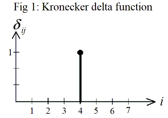
If we were to graph the Kronecker delta function, ij, the value of i would be plotted along the horizontal axis and the numeric value of ij
would be plotted on the vertical axis as shown in Fig 1 below. Here, j 4, and is held constant. Then the graph shows that when i j 4, then
ij 1,
but is 0 for every other value of i.
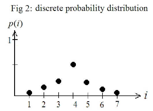
And a more general version of a discrete probability distribution might look like that in Fig 2 below, where the probability of the i th alternative is labeled p(i).
Notice that all the points are well below 1 since we need the sum of all the values for the probability distribution to equal 1,
p(i) 1.[11]
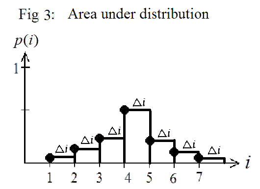
But Equation [11] can also be written as,
1 ( p(i) i )[12]
where i 1.
Equation [12]
can be seen as a sum of areas each with a width of i and a height of p(i) at various i, as is shown in Fig 3 below.
The total area after summing these up is an approximation of the area between the i-axis and the curve represented by the function p(i) from imin 1 to imax 7. More generally, however, we can make i (imax - imin) / (n -1), where in Fig 3,imin 1, imax 7,and n 7, so that i (7 - 1) / (7 - 1) 1.When i takes on successive whole numbers on the i-axis,i will always be 1 and is usually omitted.
However, what happens when we want to divide the interval, imin ≤ i ≤ imax, by a larger number of sub-intervals? This would give us a closer approximation to the area under the p(i) curve. In that case,
Equation [12] can be written as
1 p( imin + [ j-1] i )
i[13]
Here n does not necessarily represent the number of whole number steps
from imin to imax
as before. The number n could be very large in which case i (imax - imin)/n and can become
arbitrarily small as n increases. As j steps from 1 to n, p( imin + [ j-1] i ) is evaluated in increments of i along the i-axis. With arbitrarily large values of n, p(i) could be evaluated at any real value of
i, not just whole numbers. And p(i) will have to be a continuous function with a corresponding value for every real number of i
for which p(i) is evaluated.
So we must consider what happens as we let the discrete variable i become a continuous variable. When i become continuous, it's customary to label the i-axis as the x-axis,where x can take on any real value. Then p(i) becomes p(x) and must be a continuous function. The interval, imin to imax, becomes xmin to xmax,and i becomes x (xmax -xmin) / (n -1), and imin + [ j -1] i becomes xjxmin + [ j -1] x,where j still takes on values from 1 to n.
The process of integration found in the study of calculus is to let n increase without bound in
Equation [13]. We say "in the limit as n approaches infinity" and write in formulae and more simply n→ in text. And so the process of integration applied to
Equation [13] would be written,
p(xj) x 1[14]
Since x (xmax - xmin) / (n -1),as n approaches infinity, n→,x approaches zero, x→ 0.But n never actually reaches infinity since that number is really not defined. And so x never actually reaches zero, but it is increasingly small. The notation of x→ 0 is usually shortened to dx and is referred to as "differential x" meaning that it is increasingly small. And the function p(x) in
Equation [14] no longer assigns a probability for each discrete alternative as p(i) did in
Equation [11]. In Equation [14],p(x) is a probability density, assigning a probability for events to happen between x and x+dx. The notation is a little cumbersome to write, so it is usually shortened to where xmin is called the lower limit of integration and xmax is called the upper limit of integration. So changing to this
notation Equation [14] becomes
p(x)dx 1[15]
And it is call the integral of p(x) from xmin to xmax that is set equal to 1.
to an integral. This becomes necessary when the density of propositions become so dense that there is a continuous distribution of them. Using the techniques of the previous section, the continuous version of
Equation [8] becomes the integral
1, if x0 R[16]
0, if x0 R
where R is some interval on the x-axis. The function,
, is called the Dirac delta function,
and it is the continuous version of the Kronecker delta function,
ij.
The notation, ,
means evaluate the integral within the region, R, from xmin
to xmax. And instead of labeling each proposition with a discrete, whole number, i, the
density of proposition is so great that we must go to a continuous variable, x.
So the notation, x0 R,
for the Dirac delta replaces the previous notation, 1 ≤ j ≤ 2, for the Kronecker delta.
And
Equation [16]
= 1, if x0R, = 0, if not
is one of the defining equations for the Dirac delta function,
. The Dirac delta must be defined so that Equation [16] remains true independent
of the size of the region, R. Even if R is specified to be very, very small, this integral must still evaluate to 1. Therefore,
becomes very large at x0
so that when integrating, the area under the curve for
is still equal to 1 for very small R. But
is very small for any
x ≠ x0 so that
the area under the curve does not get too large when R is large.
And so the Dirac delta function is defined such that
→ at xx0, and
→0at x
≠
x0.
Both these limiting processes of → and
→0
are controlled by a single parameter, , I'll call it cap-delta. So as → 0, you get
→for xx0 and you get
→0for x ≠ x0.
This is a different limiting process than the n→ limit
for integration. One has to hold at some finite value and then do the integration on the continuous Dirac delta function,
. And then after integration is done, the limiting process of 0 is done. For it would not be possible to do the integration if one were to allow to approach infinity first. This is because times dx is not defined.
In the literature the region R in
Equation [16]
= 1, if x0R, = 0, if not
is usually the entire real line, - ≤ x ≤ +, but this does not necessarily have to be the case. Yet if R in
Equation [16] were the entire real line, then x0 would certainly be included in it, and we get,
[17]
which is mapped from the logical
Equation [9]
A→qj
=
(qi→qj) =
T, for 1
≤
j
≤
n
, = F, otherwise
and the Kronecker delta
Equation [8]
= 1 if 1 ≤ j ≤ n, = 0 if not
.
However, if R has upper and lower limits, xmin ≤ x ≤ xmax,
then the integral of
Equation [16]
= 1, if x0R, = 0, if not
is 0 when x0 R.
This is because x0
is outside the limits of integration, so
is basically 0 everywhere it is integrated. And so the integral is 0.
The intent here is to use the Dirac delta function to transform
into the Feynman Path Integral. But
Equation [7] was derived by iterating
Equation [6]
(q0→qn)
(q0→
qj)(qj→qn)
.
So if the map developed so
far to go from logic to math is indeed valid, then the Dirac delta function
should also have this same iterative property.
To that end, consider what effect
Equation [16]
= 1, if x0R, = 0, if not
would have on an arbitrary function f (x),
.
Since the function
is practically 0
away from x0 and very large
atx0, we have that f (x) is practically 0
away from x0 and large
at x0. This means we can restrict the interval of integration to a very small interval,
R', that includes x0.
Then x0 R', and R' R. And when R' becomes very small, f (x) will essentially be f (x0)if R' is a small enough interval around x0. Then the above equation becomes
.
So that we have,
for x0R[18]
But as usual, if x0R, then f (x0) will essentially be 0 throughout the
interval of integration, and
for x0R.[19]
Now x in these equations is called a dummy variable of integration, and we are free to change it to
anything we like without changing the value of the integral. So let's change the
integration variable from x to x1.Then f (x) becomes f (x1),and
becomes
,and dxbecomes dx1, and
Equation [18] becomes
for x0R.
But if f (x1) were to be a Dirac delta function itself,
, we get
for
both {x, x0}R[20]
0 for
either of {x, x0}R
Of course, now both x and x0 must be in the interval of integration, R.
Otherwise, if x R,
then
,
would be 0 throughout the integration, making the integral 0. And if x0 R,
then would be 0 throughout the integration, making the integral 0.
Note that Equation [20] is a Dirac delta representation of
Equation [6]
(q0→qn)
(q0→
qj)(qj→qn)
.
So the Dirac delta function has the same iterative property corresponding to its
logical counterpart. This is what initially attracted me to the Dirac delta
function as a math representation for implication. It took some work, however,
to justify this using the Dirac measure.
Iterating again we get,
[21]
for {x, x0}⊆ R
And iterating an infinite number of times we get,
[22]
for {x, x0}⊆ R
Obviously each ofx1, x2,..., xn
is within the interval of R since we are integrating with respect to those variables within R. And
note that
Equation [22] can be seen as the Dirac delta representation of
The mathematical map developed so far seems consistent. And we are closer to the math of
the path
integral.
To sum up, the progression has been to go from logical equations to discrete
summations to integrals,
(qi→qj)
T 1 1
.
An iterative property also follows from logic
to the Kronecker delta to the Dirac delta function,
(qi→qj)
(qi→
qk)(qk→qj)
.
All that remains is to find a mathematical expression for
that has these same properties.
There may be many functions that could be used to
represent the Dirac delta function. One such function is the gaussian form of the Dirac delta,
[23]
It has the property that as approaches zero, the delta function becomes infinite in such a way that the integral of
Equation [16]
= 1, if x0R, = 0, if not
remains one. The integration of the gaussian Dirac delta is a little tricky to prove and is done in many books on quantum mechanics that cover the path integral. (No physics is necessary in the proof.)
Here's a video of how to
integrate a gaussian function.
The gaussian Dirac delta function of Equation [23] also satisfies the
iterative property of
Equation [20]
since,
[24]
where and both act like the previous and approach zero as approaches zero. This equation is called a Chapman-Kolmogorov equation and is proved in The Feynman Integral and Feynman's Operational Calculus, by Gerald W. Johnson and Michael L. Lapidus,page 37,eq 3.2.8.
I've not found any other function that satisfies this iteration property other than the
exponential gaussian function. And it's fortunate that this integral solves the
iteration property exactly. For we need to solve the integral before we can
allow the parameter to approach zero as required by the Dirac delta function.
But if the exponential gaussian is to be used for the Dirac delta function, then notice in
Equation [23]
this makes
,
since in the exponent, 22.
Yet, x1 is stated by proposition, p1, to be the position of the
element, p1,
and x2 is stated by p2
to be the position of p2. And we
know that for material implication, (p1→p2)
(p2 → p1). So
we need to modify Equation [23] to prevent the equality when the coordinates are
interchanged.
The only parameter left to manipulate in Equation [23]is .
We need to have
depend on whether we use
or
in the
exponent of the gaussian function.
Let's start with the simple substitution 2
.
Here we are letting successive values of t mark off successive steps along
a path. So if marks off the
path, (p1→p2),
then
marks off the reverse path, (p2→p1). And
if
, then the exponent in
Equation [23]
Was,
But now is,
will be positive in the
direction but negative in the reverse
direction. And we will have
as required since (p1→p2) (p2→p1).
But since
2
,
then as 2 → 0, to form a Dirac delta, we will get
→
0.
And in the
direction, the
exponential
,
if
and
will approach infinity as →
0 since < 0 in that case. But in the reverse
direction, the
exponential
,
if
and
will approach zero as →
0since
> 0 in that case. This would seem to make the delta
representation for (p1→p2)
to be of a very different character than (p2→p1).
Not only this, but in the
direction, the
leading factor
is imaginary,
if
will be a complex number since it is taking the
square root of a negative number;
< 0.
But in the reverse
direction, the
leading factor
is real,
if > 0
will be a real number since it is taking the
square root of a positive number;
> 0. Now we have a totally different character
for one direction than another, one way is complex, the other way is real.
But it was totally arbitrary to assign which
direction through a path got greater values of t. If we
were to have assigned greater values of t in the opposite direction,
then the first direction would have been real and the second complex. Also, it's
possible to construct paths that wind about in such strange ways that (p1→p2)
could be in the forward direction in some paths and in the reverse direction in
other paths. As you construct every possible path from start to finish, each
step is used many different times, sometimes in the forward direction and
sometimes in the reverse direction. So we don't want to have steps that greatly
differ in character depending on which way you walk through them. And we don't
want to give preferential treatment to any step or group of steps. We want all
the steps to have the same character and have equal importance. For any one of
them could have just as easily been in the start or middle or end of a path.
This can be done if we modify
2 and make it 2 i,where
. Then the only difference between
and
is a phase shift.
One is the complex conjugate of the other. They are both complex, and they both
have the same absolute value. And our delta function becomes,
where m and
are arbitrary constants for the purposes here, and
.
Then we can rearrange
Equation [23] to get,
which equals
[27]
where
and
,
and where
.
Using m and
above is not an attempt to covertly introduce physics. Herem and
are constants of proportionality. It is only fortunate that they appear to be
mass and Planck's constant.
And inserting
Equation [27]
into
Equation [22]
Substitue each
with
into
to get ...
,
we get
[28]
with the appropriate limits implied, and where the R in the integrals of
Equation [22]
is the entire real line.
Since each of
,
is between t0 and t, then as
for
,
then every
for every
in Equation [22]. This is why I simply write
instead of
in the equations above. This makes all the square root factors all the same. And
we can multiply all n of the
factors together to get
. And Equation [28] becomes,
[29]
This is because the
exponents add
in Equation [28], and there is n of them, one
for each step in the path. So for any one path, j starts
from 0, the starting point, to n, the ending point. And we add them all up,
.
And as n increases without bound, there is an infinite number of t's between the start and end of the path,
so the difference between adjacent t's approaches 0. Or in other words,
.
This turns the summation in Equation [29] into an integral, and we get,
[30]
.
Notice that the
exponential factor
looks like the Action integral for a particle in motion without any force
applied. Here m and
are only constants of proportionality. Remember that the increasing direction and scaling size of t was arbitrary,
t was an arbitrary parameterization of paths. And which coordinate system to use, the positive direction and scaling of x is also arbitrary. So m and work together to cancel out whatever units occur in the integral. This is necessary because the exponent must be a pure number without units in order to evaluate it.
An exponent with units attached, like feet or seconds, doesn't make sense.
Equation [30] can be recognized as the Feynman Path Integral for the
propagator of the wave function for a free particle in quantum mechanics. The limits of the t approaching zero is
understood by the notation of dt and t.
But this formula was derived by considering how any two points in space are
connected through paths connecting every other point in space. It shows how all
of space is connected. Yet, if this formula is about space, then how can it be
about a particle which travels through space? After all, particles are different
than space, right? Yet, even with a particle, there is a starting point and an
ending point in its trajectory. And if there is no means to determine
intermediate points in its trajectory, then you are left to consider every possible
path it might have taken. So Equation [30] duplicates the math for only the kinetic energy of a particle, but what
logic might account for the potential energy of a particle? The next section
addresses this.
Now what if there were something in space which determined that implications will be stronger or weaker
at various places? Then each of the implications in a path will be weighted by a function,
?
The greater the value of this function, then the more or less effect an
implication would have in a path. The function,
, would strengthen the effect of an implication or strengthen it in the
opposite direction. In the math,
would be a factor that would be capable of changing
into its complex conjugate since the complex conjugate of an implication
is an implication in the opposite direction. So
itself would be a complex number. And instead of
,
you would have
.
Then
Equation [22]
becomes
[31]
And
Equation [27]
becomes
[32]
But since
is a complex number, we can write
,
where
.
Then Equation [32] becomes
.
Note, however, that
is never 0 or
. Again, this is so we don't create any great differences in character between
one implication and another. We don't want to give any preferential treatment to
any arbitrary points of space. So the only thing that
can do is introduce a phase shift and change the angle and possibly
reverse its direction. If
were of the right value at x, then the exponent,
,
becomes negative and turns
into something closer to its complex conjugate so that it acts more like a step in the opposite direction. But
does not change the magnitude of a step, since
.
The result of
on every possible path is to act like a potential, changing the overall
path from what it would be without it.
With
added,
Equation [30]
becomes
This is the Feynman Path Integral for a particle in a potential.
It is the wave function of a particle,
.
But what could cause a potential to occur? I have a little bit more explanation
here.
The Born rule tell us that the probability density,
,
for finding a particle between x and x+dx
that has wave function,
, is equal to the wave function times the complex conjugate of the wave function. Or in symbols,
.
This can be explained with the formulism developed here. Equation [4] is q1q2→ (q1→q2)(q2→q1)
which is an equality if at least one of q1 or q2 is true. When this is mapped in mathematical terms, each of q1 or q2 is a proposition mapped to a value between 0 and 1 depending on how likely it is. So, for example, q1 maps to a number that behaves as the probability that the proposition q1 is true. And factors like (q1→q2)
generate the path integral which is another way of describing the wave function,
. We learned that (q1→q2)
maps to a complex number, and (q2→q1)
maps to its complex conjugate. Then conjunction,
, maps to multiplication. So q1q2maps to a probability of finding q1 time the probability of finding q2, or
(q1)(q2).
The physical interpretation of (q1→q2) is that the state described by a proposition q1 leads to the state described by proposition q2. In terms of an experiment, q1 would be the setup of the experiment and q2 would be the measured result. Now, experiments are set up in a known state with certainty so that the results can be repeated. That means here that (q1) would be 1 by
deliberate design. So what we have left is (q2) equal to a wave
function
representing (q1→q2)
times the complex conjugate of the wave function
representing (q2→q1). If we let q2 be located at x,then (q2) is replaced by (x), and (q1→q2) is represented by
, and (q2→q1) is represented by
. And so we get the Born rule:
,
where must be interpreted as the square root of a probability.
The wave function expresses how one fact implies another.
But it does not give enough information to predict the probabilities of a measurement.
This is because an implication could be true independent of the premises. An
implication does not give us information about the premise. But an experiment is
specified by both the premise and conclusion, by both the setup and a
measurement. In order to form a workable hypothesis with repeatable results,
both the setup and measurement apparatus must be fully specified. You must know that the setup and the result both exist in conjunction. Otherwise you cannot form a correlation between cause and effect if you don't know what caused your effect or if you don't know what effect your cause had. So the wave function tells us what effect a cause will have, and the conjugate wave function tells us what caused an effect. And together you know both cause and effect and you can calculate the relationship (probability) between them.
And it seems only intelligence is concerned with calculating the probability between cause and effect. A screen hit by an electron doesn't care where it came from; it could come from anywhere and have the same effect. And an atom emitting a photon doesn't care what effect the photon has on any screen. Physical events don't care what the probabilities are; they simply respond to stimuli. But conscious beings with
intelligence calculate probabilities so they can make intelligent decisions.
This is likely what is meant when scientists say that observation (from
conscious beings) collapses the wave function to the measured result. It is only
conscious beings that form correlations between proposed causes and effects.
The quantum mechanics of the wave function
(or path integral) is usually called 1st quantization. Functions are obtained with this procedure. There is also a branch of quantum physics called quantum field theory which is sometimes called 2nd quantization. It takes the fields obtained in 1st quantization and plugs them into a very similar quantization procedure to get 2nd quantization. Again, it seems like there is little justification for further quantizing fields other than it just so happens to predict results. It occurs to me, however, that quantum field theory comes naturally to the procedure described here.
We started with the fact that
qi→
(qi→
qj)
[5]
which is an equality if at least one of the qi is true. And so it became necessary to evaluate
(qi→qj)
(qi→q)(q→q)...(q→qj)
[7]
which when represented in mathematical form became the path integral of 1st quantization.
But there is no reason not to apply Equation [5] again to get
qi→(qi→qj)
→
((qi→qj)
(qk→ql))
,
in which the last conjunction is an equality if at least one of the (qi→qj) is true, which will be the case if at least one of the qi is true. And if we let qij = (qi→qj), then we have
qi→
(qij→qkl)
.
And likewise, this would necessitate the evaluation of
(qij→qkl)
(qij→q)(q→q)...(q→qkl)
In this case the mathematical representation of (q→q) would be
,
where
is the wave function of 1st quantization and is the mathematical representation of q (q→q).
The delta here would be expected to still be an exponential gaussian with
replacing xi
in the exponent. And d would replace dx in the integrals to finally get
,
which is the path integral of 2nd quantization used in quantum field theory.
And I suppose the same procedure can be used to get 3rd quantization except that keeping track of the indices might be tedious.
Previously the complex numbers were used in the wave function of 1st quantization. And the complex numbers establish the U(1) symmetry of QED. I have to wonder if a similar effort for the four numbers associated with the
(q→q) of second quantization or the eight numbers associated with third quantization might establish the quaternions or octonions used in the quaternionic representation of Isospin, SU(2), or the octonionic formulation of SU(3) used in particle physics. I am by no means an expert in these matters. I only
noticed their use in my reading, and now it seems they may become relevant. John Baez has a brief introduction to quaternions and octonions here. There the iteration from complex numbers to quaternions to octonions is very similar to the iteration from first to second to third quantization here and suggests their use. Further references on quaternions and octonions of symmetry groups in physics are here and here.
Having noticed a parallel between paths constructed from logical implication and paths constructed of particle trajectories, I extended that analogy to reconstruct Feynman's Path Integral from simple logic. The conversion is achieved by representing the material implication of logic with the Dirac delta function and then using the complex gaussian form of the Dirac delta. However, at this point my derivation has not been reviewed by reputable sources. It has yet to pass inspection by mathematical logicians. Until that time, this effort should be considered preliminary.
I may not have given a full account of all of the quantum mechanical formulism yet. I've not derived Schrodinger's equation, eigenvalues and eigenvectors, Hilbert or Fock space, or Heisenberg's uncertainty principle, for example. But I suspect that the rest may
be implied by the wave function that I have derived. For example, the Schrodinger equation is derived from the path integral in many quantum mechanics text.
The uncertainty principle is derived from the wave function integrated with the
Fourier transform of it. And the uncertainty principle can also be derived from
the operators for the measurements involved. So you might get operators from the
the uncertainty principle.
Keep in mind that I'm not claiming to have derived all of physics from logic. In order to claim a logical derivation of physics, one would have to derive physical quantities such as some of the 20 or so constants of nature or the principles of General Relativity. So I will keep an eye on such efforts. And I'll try to include more as time and insight allow.
However, this does open an intriguing possibility for deriving the laws of nature. Typically physicists use trial and error methods for finding mathematics that describe the data of observation in very clever ways. These theories are then used to make predictions that experiment may confirm or falsify. When very many observations are consistent with the equations, we have confidence that the theory is correct. However, such theories can never be proven correct and are always contingent on future observations confirming them. But we can never say they are completely proven true. For we don't know whether some observation in the future may falsify the theory. Now, however, there may be the possibility that physical theory can be derived from logical considerations alone. Such a theory would in essence be a tautology and proved true by derivation. We would have to check our math against observation, of course. But if even one observation was consistent with such a theory, how could we say that other observations would not be? Can we expect that some parts of nature are logical but others are not when they coexist in the same universe?
We may not have any choice but to derive physics from logic since the ability to confirm ever deeper theories will require energies that are beyond our abilities to control. After all, we cannot recreate the universe from scratch many times over in order to confirm some proposed theory of everything. So we may be forced to rely on logical consistency alone. And I think I have a start in that direction.
Now, having derived the transition amplitudes of a particle from
logic alone, I use these transition amplitudes in a description of virtual
particle pairs. These virtual particle pairs come directly from the conjunction
of points on a manifold and can be used to describe many of the phenomena we see
in nature, perhaps all. For more details see this article.
If you'd like to leave a comment, please feel free to do so.

 (qi
→ qk)(qk
→ qj) [6] }
(qi
→ qk)(qk
→ qj) [6] }  ik
ik . The next section gives a brief
introduction to integration.
. The next section gives a brief
introduction to integration.