Deriving the Particles
Here I derive the particle content of the framework developed here. And it will be seen to be very similar to the particle content of the Standard Model. I will not attempt to get the quantitative mass or charge or spin values of the particles. I only attempt to give the number of particles and the comparative levels of charge for the electron and positron, the Weak force bosons, the quarks and the gluons. I also give some indication where the photons and neutrinos come from. I also give some explanation for the three mass generations.
As I show elsewhere, the transition amplitude of a particle can be obtained from first principles. The complex conjugate of this is interpreted as the antiparticle partner. Since there are only two amplitudes that can be obtained from a complex function and its conjugate, this matches the expectation for the electron and positron of the Electromagnetic force. Armed with this perspective a 2nd iteration of the formulism will be shown to duplicate the properties for the W and Z bosons. The 3rd iteration will seem to replicate the number of particles and charge levels of the quarks. Iterating again gives us what appear to be gluons.
If the formulism developed here is correct, then this may possibly provide means of specifying wave functions for W and Z bosons and the quarks, etc. This may help explain why the Weak bosons are so short lived and why the quarks are confined. It may also give means of calculating the relative masses of the particles. The exact nature of interactions and decay might be discerned. And it may also give means of calculating the coupling constants from first principles.
INTRODUCTION
In summary, the previous article
starts with the assumption that reality consists of a collection of things all
coexisting in conjunction with each other. Space itself consists of a
conjunction of points, where each point is described with a proposition stating
its coordinates. This results in Equation [3], shown below, where each
![]() [3]
[3]
However, a conjunction between two points results in implications between those points, as shown in Equation [4] below.
![]() [4]
[4]
So a conjunction implies an implication both ways. And this means that the conjunction of all the points in space implies an implication between any and every two points of space, as expressed in Equation [5] below.
![]() [5]
[5]
This makes it necessary to study what it means to have an implication within a conjunction of points. And it was discovered that such an implication equates to a disjunction of a conjunction of implications as shown in Equation [6] below.
![]() [6]
[6]
This is a recursive relation that can be iterated any number of times. And when iterated an infinite number of times, Equation [7] is derived as shown below.
![]() [7]
[7]
This is a disjunction of many terms. Each term is a series of implications that
represent a path of steps from start to finish. Since each of the i's in the
disjunction runs from 0 to n, Equation [7] represents every possible path from
However, implication can be expressed in set
theory by the relation of subset. If B is a subset of A, then if A exists, B
also exists, but not the other way around. And a numeric value can be assigned
to the relation of subset using the Dirac measure,
x(A), which is equal to 1 if x is included in A and is 0
if x is not in A. This allows us to map a true proposition a value of 1 and a
false proposition a value of 0. If the set A of the Dirac measure is reduced to
a single element, then the Dirac measure reduces to the Kronecker delta,
![]() [20]
[20]
This equation can also be iterated an infinite number of times, as shown in Equation [22] below.
![]() [22]
[22]
The complex, Gaussian exponential version of the Dirac delta function is used, as shown below.
![]() [27]
[27]
And this can be shown to solve the recursive property of Equation [20]. When the equation above is substituted into Equation [22], we get,
![]() [28]
[28]
The exponents of this equation can be manipulated as follows,
And when this is substituted into the last integral above, we can collect the exponential terms to get a summation. And we can combine the square-root factors to get Equation [29] below.
![]() [29]
[29]
Now in the case of a continuum, as and , the summation above becomes an integral and we get Equation [30] below,
![]() [30]
[30]
.
This is Richard Feynman's Path Integral of quantum mechanics for the trajectory of a particle free of any forces acting on it. Again, the details of this derivation are covered in the previous article.
The path integral is another way of obtaining the wave function. It is also called the transition amplitude. Obtaining the wave function is this manner may seem like a trick of mathematical manipulation. But if the particles of the Standard Model emerge from this framework, then perhaps this deserves more attention.
FINDING PARTICLES
The last section gives us a starting vocabulary and basic framework. The goal now is to recognize the particle content of this formulism. Shouldn't we expect that the underlying principles that give us quantum mechanics would also give us the particles to which it applies?
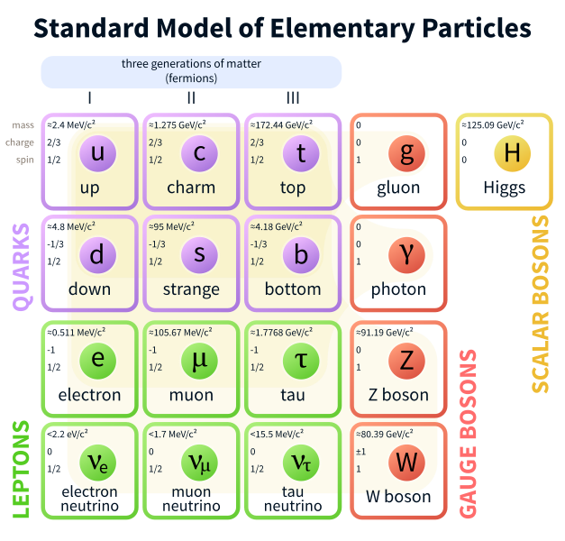
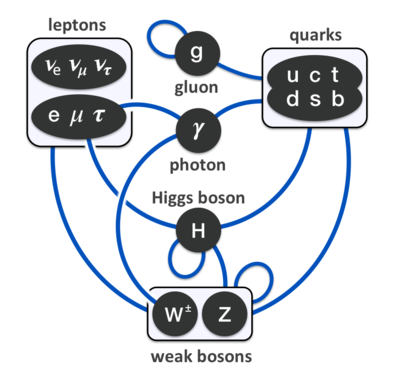
The Standard Model of particle physics describes about 17 fundamental particles. There are bosons and fermions, quarks and leptons; the fermions have 3 generations of mass. There is the Higgs boson, and the charged particles have their antiparticle. The table below to the left shows how the particles are arranged. The diagram to the right shows how they interact with each other. These particles make up all the atoms and molecules we see. And the trick will be to find them hiding in the logic of this framework. The attempt will be to show that the particles of the Standard Model can be matched to characteristics of this formulism.
Previously, I suggested that the implication between points could be expressed with complex numbers which was responsible for giving us the particles of the electromagnetic force. And when iterated, the implication between implications would give us the particles that participate in the Weak nuclear force. And when iterated again, the implication between the implication of implications would give us the particles of the Strong nuclear force. This all seems a bit abstract, and so now I'd like to flesh this out.
Because a conjunction implies an implication both ways,
![]() [33]
[33]
And the reverse implication,
But Equation [33] is also the expression for the transition amplitude for a particle,
![]() [34]
[34]
and the transition amplitude for the antiparticle is expressed by the complex conjugate,
![]() [35]
[35]
where
.
This is possible because an antiparticle can be thought of as a particle traveling backwards through time. It seems to be a time reversed version of a particle. But time reversing the transition amplitude is the same as taking the complex conjugate without time reversing. Time reversing means taking the negative of . If represents a particle moving forward through time, then represents an antiparticle moving backwards in time. Yet, since is a cofactor with the i in the exponent and in the square-root of the transition amplitudes, we can transfer the negative sign on and put it in front of the i to get the complex conjugate. Then the complex conjugate of the transition amplitude represents an antiparticle traveling between the same two points in the same period of time, where both particle and antiparticle are now moving in the forward direction of time.
To be concise, the conjunction of all points in
space results in an implication between every two points. And there is nothing
to distinguish one point from another, except arbitrarily assigned coordinates.
So there should be nothing to distinguish one implication from another. One
implication is just as valuable as another. But an implication one way is not
equal to the implication the other way,
Now the electromagnetic force acts on two charged particles, the electron and the positron. And since my math representation of implication and its reverse implication is equivalent to the transition amplitude of a particle and antiparticle, this suggests that implication and its reverse, represents an electron and positron, since one is the complex conjugate of the other.
So I will identify the charges of particles with the unique different ways to configure the various implications within an iteration. The 1st iteration has 2 configurations, an implication and its reverse, and is interpreted as the positive and negative electric charge of the positron and electron. The 2nd iteration is characterized by the implication between implications, and there are 4 different ways to configure the implication between implications and their reverse, 3 of which are unique. These are interpreted as the W +, W -, and Z 0 particles of the Weak nuclear force. The 3rd iteration is characterized by the implication between the implication of implications, and its reverse, 5 of which are unique. These will be interpreted as the up, anti-up, down, anti-down flavor property of the first generation quarks. The second and third generation particles will be just a little more difficult to explain. There is also a fifth quark with zero charge found here; this is not found in the Standard Model. But some think it may explain dark matter. And finally iterating again, there seems to be 8 unique configuration which can be interpreted as the 8 different gluons. Photons and neutrinos are interpreted here as special ways of combining previous particles.
As you may have guessed, I'm using italic words to indicate my interpretation of my formalism since they seem to match the properties of the Standard Model.
THE WEAK ITERATIONS
In the previous section, the forward implication is represented with the complex, exponential gaussian function.
And the reverse implication is represented by its complex conjugate.
We can abbreviate this to
and
if we let and .
A graphical representation of the transition amplitude and its conjugate are shown below in Fig 1A and Fig 1B.
The p of Fig 1A and the e of Fig 1B are continuous functions of space and time. The arrow in Fig 1A indicates that the p transition is from xp to xq as time increases. So here it is easy to see in Fig 1B that the e transition travels backwards in time from xq to xp and, therefore, is the antiparticle of the p.
We then get two mathematical entities in the 1st iteration of the framework. Because this seems to equate to the transition amplitudes of a particle and antiparticle, I somewhat arbitrarily identify the forward implication of the logic with a positron and the reverse implication with an electron. To avoid making controversial claims, I will use italic words to label my interpretation of my framework and non-italic words to refer to the particles of the Standard Model. What I hope to show is that the number of particles with the various kinds of charge can be accounted for.
Now implication is a part of the 1st iteration of this framework. But if implication and its reverse can be identified as a positron (p) and electron (e), then the question becomes do the iterations of this formulism correspond to particles of the other forces of nature. Let's do the iterations and count the particles.
In the 1st iteration, a conjunction of two
points gives us an implication both ways,
In the 1st iteration, implication was represented by the Dirac delta function, which is manipulated into the transition amplitude of Equation [34],
.
The reverse amplitude is accomplished by interchanging xp and xq while at the same time interchanging tp and tq. This makes the reversed amplitude equal to the complex conjugate of the forward amplitude. And since a complex number is not generally equal to its complex conjugate, the reversed is not equal to the forward amplitude. So we interpret this to be two distinct particles, a positron and an electron.
The 2nd iteration is accomplished in the logic by replacing the propositions in the 1st iteration with implications. In the math this means replacing the coordinates xp and xq with transition amplitudes. If the transition amplitudes are for positrons, then we would make the following substitutions in Equation [34].
![]() [36]
[36]
![]() [37]
[37]
If the transition amplitudes were for electrons, we would substitute,
![]() [38]
[38]
![]() [39]
[39]
Or we could substitute any combination of electrons or positrons. Substituting
two positrons, we would get the amplitude,
![]() [40]
[40]
Now things are getting more complicated. Instead of the single exponent we had in the 1st iteration, we now have exponents inside an exponent in the 2nd iteration. This gives us amplitudes inside amplitudes. So I will use colors to distinguish the different iterations; black is for the 1st iteration, magenta is for the 2nd iteration, and aqua is for the 3rd iteration. These colors have nothing to do with the color charge of the Strong force.
Notice in Equation [40] that there is an imaginary number, i1, in the 1st iteration part (the black text), but there is a different imaginary number, i2, in the 2nd iteration part ( the magenta text). These two imaginary numbers, i1 and i2, are responsible for making the amplitude of Equation [40] a quaternion number. I'll define quaternions a little later on this webpage.
Also notice that I've made a distinction between me and mz in the 1st and 2nd iterations. I don't know that they have the same value, though they might. And lastly, I will use lower-case English letters as indices to distinguish spacetime points, and I will use lower-case Greek letters as indices to distinguish individual particles.
If we use definition of Eqp and Aqp above, Equation [40] can be abbreviated to,
.
With similar definitions for and , this can be further abbreviated to,
![]() [41]
[41]
We can make a graphical representation of Equation [40] in space and time as shown in Fig 2.
The black arrows represent the 1st iteration math written in black. The magenta arrow represents the 2nd iteration math written in magenta. Here we see two positrons, traveling forwards in time, connected to each other. Keep in mind that everything pictured here is at a small, differential scale. The black math of Equation [40] came from the Dirac delta function in Equation [27], which is integrated in Equation [22]. So the math in black is a differential. Consequently, the magenta math in Equation [40] is a differential that must also be integrated to find a wave function. And since everything is differentially small, it can be represented as a point particle, and we can imagine space potentially being filled with a field of these real or virtual particles.
But it will be easier to simplify Fig 2 to the graph shown in Fig 3.
Then we can talk about the number possible combinations of e's and p's and the forward and reversed versions of them.
For example, if the particle in Fig 3 represents the forward
implication,
If Equation [40] represents the forward amplitude, then the reverse amplitude is obtained by reversing the order of and and reversing the order of subtraction in the exponent. This give us a reverse amplitude,
But since , we can keep the original order of subtraction in the exponent. And we can also keep the original order of and if we take the complex conjugate of . So in terms of the abbreviated version, if the forward amplitude is,
then the reverse amplitude is,
Technically, the reverse amplitude is not mathematically equal to the forward amplitude. So the asymmetry between forward and reverse implication maps to an asymmetry between the forward and reverse amplitude as required. But notice that . So we can make . Then we can distribute the between the two 1st iteration exponents to get,
In other words, the minus sign in the 2nd iteration exponent only adds a phase angle to the 1st iteration amplitudes. And both terms inside the square are shifted by the same phase. However, according to this article, a phase factor gets cancelled out in the calculation of any expectation value. So a phase factor does not have any physical meaning. And both terms inside the square still essentially represent a positron as before.
Similarly,
Again, this phase factor is physically meaningless. The resulting particle is essentially the same as with no minus sign. So what is shown is that the forward and reverse implication in the 2nd iteration is actually the same particle. This result applies to every combination of electrons and positrons substituted in Equation [40].
Also, notice that if the forward implication of
then the forward implication of
Although these two amplitudes are not mathematically equal, they are essentially the same particle, since either way you look at it, it is still connecting a positron with an electron.
So out of the many possibilities that we started with in this Section,
For
This particle has a negative electric charge, so I tentatively label it as a .
For
This particle has a positive electric charge, so I tentatively label it as a .
For
This particle has no electric charge, so I tentatively label it as a .
Thus, the 2nd iteration seems to account for the W and Z bosons of the Weak nuclear force. We have the correct number of particles and the same positive, negative, and zero levels of charge. The only difference is that the Standard model has a -1e charge for the W- and a +1e charge for the W+, whereas I get ±2e. If I were to divide by 2, I would get the same electric charge as the Standard Model for the W and Z bosons. So notice that if I were to ignore the plus or minus sign of the charge I get and only count the different absolute magnitudes, |0e| and |±2e|, there would be two different levels. If I divide by the number of different absolute values, there are 2, I would get the same electric charge for my weak bosons as the Standard Model. This trick also works in the 3rd iteration described below. I don't know why this trick would work. Perhaps there is a group theoretic reason, or perhaps it occurs by taking into account superpositions of states. Other reasons that the charge would be ±1e instead of ±2e might be perhaps the connection in the 2nd iteration acts like a positive charge reducing the overall negative charge in the , and similarly for the . Or perhaps there is some unusual screening of the electric charge due to the 2nd iteration connection. Or perhaps the electrons and positrons in these particles are closer to being virtual and don't acquire the full charge of an electron or positron.
It's curious, though, the Standard Model considers the W and Z bosons to be elementary particles, not consisting of constituent sub-particles. But these Standard Model particles can decay into electrons, positrons and neutrinos with a probability determined by a coupling constant derived from experimental data. However, the and bosons derived here are made of constituent sub-particles, the electron and positron. So here it is easier to see how such decay modes are even possible. The primary means of propagation comes from the electrons and positrons since their transition amplitudes are functions of time and space. And the propagation of these constituent electrons and positrons are constrained in order to maintain the connection of the 2nd iteration that defines those particles. The likelihood of the W and Z bosons to decay might then depend on how far the and Z particles can travel without losing their particle-like propagation characteristics.
Consider the 2nd iteration forward amplitude for a particle shown again below (Equation [40]).
The math in black is an amplitude for the propagation of a particle. When integrated with the path integral, this results in a wave function for a particle that propagates through time and space indefinitely with a given velocity. But the whole of Equation [40] will also need to be integrated with the path integral to result in the wave function for a . The integration should be doable, since the differential of what's inside the square of the exponent is include in the integrand. This allows the integral to be treated as if it were the integral of a gaussian. So we should get a similar form as Equation [40] for the wave function for a , with exponents inside exponents.
The question is how does a wave function propagate that has an exponent inside an exponent? I suppose that there is an approximation that can be made near the start of the propagation that appears to look like the normal wave function to which we are accustomed. But farther away, with increasing time, this approximation is no longer valid and second order affects make the wave function diverges, possibly into other particles. Decay rates might be discernable in this equation.
Furthermore, it's obvious that these and bosons are more massive than the electron or positron simply because each one is constructed of 2 electrons and/or positrons, and a heavier mass for the W and Z bosons is what we find in the Standard Model as well. I've written a different mz than for me, but we might naively expect them to be the same if we simply iterate without concern. If so, then the starting approximation for a weak force particle amplitude may have a starting mass term that might be calculated from Equation [40]. And so we might be looking at a means of reducing the number of independent constants of nature.
Now that we appear to have derived the W and Z bosons, we can move on to consider the quarks. All the techniques developed in this section will be applicable to quarks as well.
THE STRONG ITERATIONS
The 1st iteration of this framework gives us what appears to be electrons and positrons. The 2nd iteration gives us what appears to be and bosons. We might expect the 3rd iteration to give us what appears to be quarks. In this Section I show how iterating again will give us up and down quarks and their antiparticles. In a later Section I show how the other generation quarks can be obtained.
In the 1st iteration the
conjunction of any two points in space results in an implication between those
points and the reverse:
The 2nd iteration is obtained
by replacing the proposition,
The 3rd iteration is obtained
by replacing the propositions,
{[(r
→ s)
→ (t
→ u)]
→ [(v
→ w)
→ (x
→ y)]} {[(v
→ w)
→ (x
→ y)]
→ [(r
→ s)
→ (t
→ u)]}.
In the math, the 1st iteration maps implication to a transition amplitude,
In the 2nd iteration math, these amplitudes themselves are reinserted the amplitude, one for each of the variables. This gives us:
The math in black is the 1st iteration; the math in magenta is the 2nd iteration.
Likewise, in the 3rd iteration math, we reinsert the last equation for each of the variables in an amplitude. This gives us:
![]() [42]
[42]
And this is even more complicated. Now we have amplitudes inside amplitudes inside amplitudes. But with the appropriate definitions for E and A and W and B and Q and C, this simplifies to:
the aqua is for the 3rd iteration math.
And the space-time graphical representation of Equation [42] is shown in Fig 8.
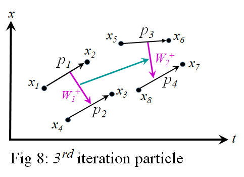
The p stands for positrons, and the stands for the Weak bosons. The black arrows are for 1st iteration particles of electrons and positrons. The magenta arrows are for 2nd iteration particles of and bosons. And the aqua arrows are for 3rd iteration particles which will turn out to be the quarks.
Fig 8 can be simplified by drawing it in 1st iteration particle space as shown in Fig 9 below.
And this can be simplified even further when drawn in 2nd iteration particle space as shown in Fig 10 below.
In the previous section, the 2nd iteration and bosons were shown to be the only unique combinations of 1st iteration electrons and positrons that were possible to connect with a given charge. All the other combinations reduced to one of these. So in order to count the 3rd iteration particles, all we need do is consider all the unique combinations of 2nd iteration particles that can be connected. As usual, their uniqueness is classified by the levels of charge. And again, in particle space we don't have to consider the direction of the arrows; one way only adds a phase angle to the amplitude of the other way and has no physical importance.
Using the methods of the previous section, let and have an electric charge of +1 and 1, respectively. And the has an electric charge of 0. Then Fig 10 above has the highest possible charge. So I tentatively label it an up quark, . It seems to have a charge of +2.
Next, consider connecting a to a as shown in Fig 11 below.
This particle has the lowest possible charge of 2. So I tentatively label it an anti-up quark, .
And there are other possible levels of charge. Consider connecting a to a as shown in Fig 12 below.
This particle has a charge of 1. So I tentatively label it an down quark, . Its antiparticle is shown below in Fig 13.
This particle has a charge of +1. So I tentatively label it an anti-down quark, .
However, there are also combinations of and bosons that have zero charge as shown in Fig 14.
These particles are electrically neutral with zero charge. I label it a , which is the Greek letter sigma used at the end of words. I only use this symbol because it somewhat looks like a fancy Z for zero charge. The two particles of Fig 14 are indistinguishable and represent one particle. Since it has zero charge, it is its own antiparticle.
So the list of quarks obtained from this framework are the , , , , and the , with charges +2, 2, +1, 1, and 0, respectively. These are supposed to represent the property of flavor for the first generation quarks. If I use the trick from the previous section, I should divide these charges by the number of different absolute values. There are 3 of them, |0|, |±1|, |±2|. So if I divide these charges by 3, I get +2/3, 2/3, +1/3, 1/3, and 0. And this matches the electric charge for the quarks of the Standard Model. Except there is no quark in the Standard Model that has 0 electric charge. This is beyond the Standard Model. However, some have suggested that perhaps dark matter could consist of a quark with 0 electric charge, here. And there is talk about such a singlet quarks being needed for grand unification scenarios, here.
But quarks also have what is called a color property of red, green, blue, or anti-red, anti-green, or anti-blue. The color property does not have anything to do with frequency of visible light. These are just archaic names given to this property of quarks. The discipline of Quantum Chromo Dynamics (QCD) studies this property of color; this is what is responsible for the Strong nuclear force that binds quarks, protons, and neutrons together in an atom.
So the question is can we find 3 configurations and their reverse hiding in each quark of this framework. It turns out that we can. For there are different ways to connect the electrons and positrons that make up a quark of a given charge. For example, consider the ways we can make anti-up quark, . The first way is shown in Fig 15A.
Then second way is shown in Fig 15B. And the third is shown in Fig 15C. All these configurations have the same electric charge, and they have the same Weak isospin charge. So all these configurations should interact with the other particles in the same way. But they are mathematically different since in the 1st iteration each is connecting different space time points in Equation [42]. And the same can be said for the quarks, since we only change p's for e's and for .
Similarly, the electrons and positrons of all the other quarks of a given electric charge can be connected in 3 different ways. And since there is no way to measure which configuration a quark is in, all 3 configurations exist in superposition for each quark. Which configuration a quark is connected really does not matter except when you are connecting one quark with another as is done in the 4th iterations with gluons as described in the next section. For then we draw an orange arrow from one aqua arrow to another aqua arrow. And since the aqua arrow changes with configuration, the orange arrow will be interrupted until reestablished.
So perhaps the 3 different ways of connecting the underlying electrons and positrons gives us the 3 different colors of the Strong nuclear force. Then the anti-colors could be obtained by reversing the aqua arrow in a quark. If so, the question becomes why does this create such a strong force between the quarks? I don't know at this point.
But it does seems intuitive that the quarks should be heavier than the and bosons since they are constructed of more electrons and positrons. And it seems obvious that the quarks should operate on a smaller scale than the Weak bosons since the math of Equation [42] has an extra exponent to make the equation diverge more quickly from an approximation.
Gluons
If we iterate again, we can use the same methods. We simply count the number of ways that the previous iteration particles can be connected with unique electric charge. In the 4th iteration we find the number of way to uniquely connect 3rd iteration particle. We will find that there are nine of them.
In Section 4 we found the quarks with the various flavor and color charge. These are:
→ , anti-up, 2/3e
→ , down, 1/3e
→ = → , zero, 0e
→ , anti-down, +1/3e
→ , up, +2/3e
Now let's list every combination of quarks with unique charge:
→ , 4/3e
→ , 1e
→ = → , 2/3e
→ = → , 1/3e
→ = → = → , 0e
→ = → , +1/3e
→ = → , +2/3e
→ , +1e
→ , +4/3e
Here we seem to have nine gluons. The Standard Model also has nine gluons, two of which combine into one state, giving eight distinct gluons. Fig 16 below shows the eight gluons as black dots. The colored triangles labeled with a q represent quarks; the upward pointing triangle are quarks with red, greed, and blue color charge, the downward pointing triangles are antiquarks with anti-red, anti-green, and anti-blue color charge. Here is a short video about quarks and gluons that might be helpful.
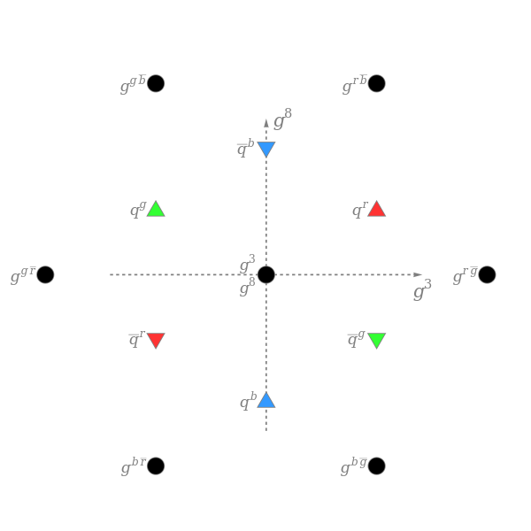
Fig 16: Types of gluons and quarks
However, the Standard Model gluons have no electric charge whereas those developed here do. However, if I divide by the number of distinct absolute values as I did in the previous sections, there are 5 of them, |0|, |±1/3|, |±2/3|, |±1|, and |±4/3|, then I divide by 5 and get a much smaller charge. Perhaps this is small enough not to have been detected so far.
The Standard Model gluons also have no mass whereas those developed here would seem to have a huge mass, more than the quarks. Yet, there might be a means of propagation where the mass converts to a frequency of propagation at the speed of light.
Or, a 4th iteration may not be the way to get gluons and we must look for a different mechanism that gives us gluons. The effort to find gluons so far has not taken into account the different configurations of quarks that I have labeled the color charge. And a more direct consideration of these color configurations may be what is needed.
If quarks can be connected, one possibility is shown in Fig 17.

But there are other ways to connect quarks, depending on their color configuration. Another way is shown in Fig 18 and Fig 19, where we have changed the color configuration of only the left quark.
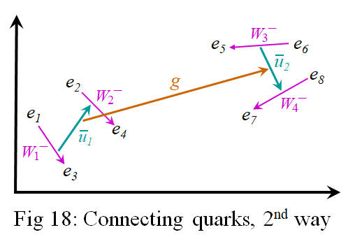
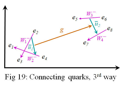
And we can also change the color configuration of the quark on the right. In fact, there are 3 color configurations of the quark on the left for each of 3 color configurations of the quark on the right. Again, this is a total of nine, 3 of which leave both sides unchanged if that type of connection should occur again. Perhaps these represent the 3 color-anticolor gluons of the Standard Model that leave the quark color unchanged if exchanged.
All these possible ways to connect quarks exist in superposition with each other. And the complex phase of things that exist in superposition can interfere constructively or destructively. It's possible that they can add to each other or cancel each other out. But in the context of connecting quarks, every possible connection is of the same length scale. So the phase angles would have more of a tendency to add than to cancel out. So all these ways of connecting quarks would seem to only strengthen the connection between them. Perhaps this is the reason that the color force is so strong between quarks.
But how can mere connections from one quark to another be considered a gluon particle? In Quantum Field Theory, particles propagation can be described with Feynman's Path Integrals. But Feynman's integral has a perturbation expansion which takes into account every possible intermediate exchange with virtual particles. So if this connection between quarks can be mediated with every possible virtual process, then it is equivalent to the propagation of a particle. So I need to explain virtual particles in the context of this framework. Then I can show how the connections explained here are actually particles in the quantum mechanical sense. This is the subject of the next section.
However, first notice that there are other ways of connecting the electrons in Fig 17 (repeated below).
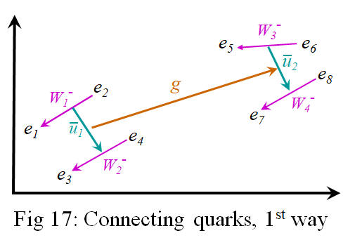
Notice here that e2 is close to e5 and e4 is close to e7. So it's possible to break all the previous connections and to connect e2 and e5 into a and e4 and e7 into a and then to connect these into a quark. But this would leave e1, e3, e6, and e8 unconnected. In order to maintain (conserve) the weak charge, flavor charge and color charge, these unconnected electrons would have to connect to each other to form their own quark, or they would have to combine with some other nearby quark to conserve all charges. This is a more traumatic reordering of things, so it's probably less likely to occur. But there are many more ways of recombining them, so it may result in a stronger connection. I wonder if this is the origin of quark confinement.
Virtual Processes
Many of the processes in quantum theory can be explained in terms of virtual particles. Virtual particles appear out of empty space, they appear for a very brief moment, and then they disappear back into empty space. They appear in pairs from a single point, as particle and antiparticle; they each travel an arbitrary distance to the same place where particle and antiparticle meet up again and cancel each other out. And this process of cancelling each other out results in their having no permanent effects. The virtual particles do not continuously propagate like normal particles. So in that sense they are not considered real. But they can interact with each other and with real particles, so they can change the trajectory of real particle. Yet where do the virtual particles come from?
Virtual particles appear naturally in this framework. In a
previous article, I describe how virtual particles
are the result of all the points of space all coexisting in conjunction with
each other. This conjunction of all points means that there is a conjunction of
any two points of space. So recall that
a conjunction of any two points results in an implication between those points
along with its
reverse implication,
The point is that there are virtual particles everywhere in space at all
times. Virtual particles can travel from any point to any other point and
interact with real or virtual particles in the process. The conjunction of all
points mean there is an implication and its reverse everywhere in space. These
are interpreted as virtual electrons and positrons that exist everywhere.
And if the conjunction of all points necessitates implications everywhere, then
we have a conjunction of implications which necessitates implications of
implications everywhere in space as well. These implications of implications are
interpreted as virtual
For example, consider how an electron might propagate from an initial position, pi, to a final position, pf. Since the two points, pi and pf, both exist in the manifold of space, there are virtual electrons and positrons with transition amplitudes from those two points. Since virtual particles can interact with real particles, the real electron at pi could cancel out and annihilate with the virtual positron of a virtual electron/positron pair. But this leaves the virtual electron of the pair unable to cancel out with its partner; it become a real electron at pf. In other words, the electron at pi has travelled to pf. For what remains of this interaction is a transition amplitude of an electron from pi to pf. This is the most direct path from pi to pf, but there could be other paths with more intermediate steps.
The electron initially at pi could interact with a virtual pair going from pi to p1. The electron would annihilate with the positrons of the virtual pair, leaving the electron of the pair to become a real particle at p1. And then this electron at p1 might interact with a virtual pair going from p1 to p2, resulting in an electron at p2. And through a series of virtual particle trading, the electron is seen to jump, step by step, from pi to pf. So in this way it is possible to construct a path of any number of steps from pi to pf. Every possible path must be considered in the math. And this in essence is the math of Feynman's path integral described in the introduction above.
Particles seem to travel through a series of interactions with virtual particle/anti-particle pairs. This works for the electrons and positrons, but it should also work for Weak bosons, quarks and gluons since they also have anti-particles that form virtual particle/anti-particle pairs. The particles that do not have an anti-particle are electrically neutral; they are their own anti-particle and so do not need to be paired with a virtual partner.
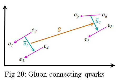
But virtual particles aid in more than the interaction which define the propagation of a particle. Virtual particles also aid in the interaction of various kinds of particles with other kinds of particles. Remember how quarks were connected by a gluon as shown again in Fig 20. Here the quarks, u̅1 and u̅2, are connected by gluon, g. This is one way a quark and interact with another quark.
But there are other ways one quark can interact with another. For instance, a virtual quark/anti-quark pair could emerge for a moment out of the vacuum as shown in Fig 21.
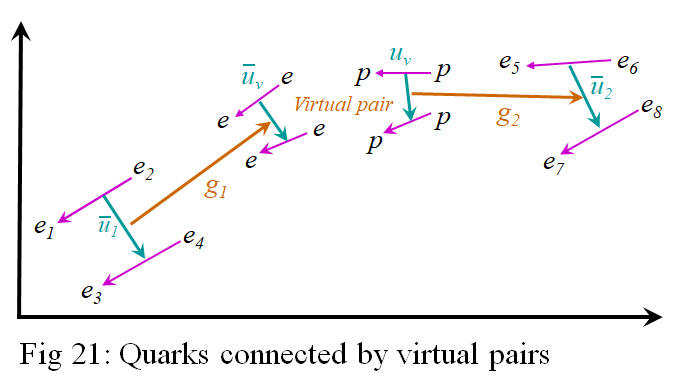
Here, u̅v and uv are a virtual up/anti-up pair. They are created at the same time at the same place, they exist long enough to establish gluon connections, then they annihilate. The connection from u̅1 to u̅2 is from g1 through the connection of the Virtual pair and then through g2. This is another way to connect two gluons. And there could be many virtual quark pairs connecting u̅1 to u̅2, with each virtual pair connected by gluons to the next virtual pair. And of course, we would have to take into account every possible way to connect the gluons in order to calculate how the gluons propagate.
The other particles
The particles explained so far are the most general interpretation of the implications. The end points of the connections have the most freedom; each is different from the others. However, other kinds of particles can be constructed if some of the end points are shared in common. For instance, Fig 22 shows the spacetime configuration for a particle.
Notice that each of the spacetime points, x1, x2, x3, and x4 is an independent point, separate from the others. But suppose we make x2 and x4, to be a common point. Then we have the configuration shown in Fig 23.
The exponential part of the amplitude for Fig 22 is shown in Equation [43].
![]() [43]
[43]
But if x2 and x4 are the same point, then Fig 22 becomes Fig 23, and Equation [43] becomes Equation [44].
![]() [44]
[44]
Here t1
< t2 and t2 < t3. So Fig 23 represents an electron starting at x3 and moving to x2, and then after that, moving from x2 to x1. Remember that an electron moves backwards in time. Fig 22 has two electrons existing at the same time; it represent the logical expression,But could e1 of Fig 23 be changed into a positron, p1, as shown in Fig 24?
Here, both the electron and positron are meeting together at x2. I suppose they would immediately annihilate each other before they could be connected into a single particle. So I don't think this particle can even exist.
Consider, however, the spacetime configuration of an Up quark as shown in Fig 25.
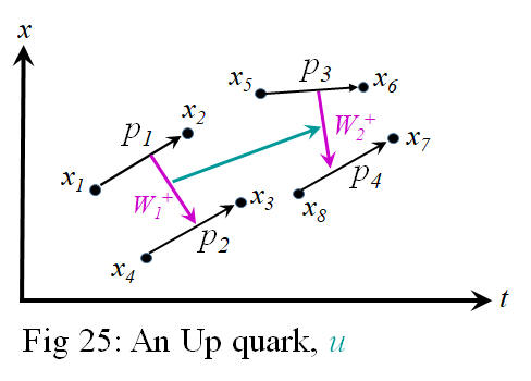
If x4 = x2, and if x3 = x5, and if x8 = x6, then we would have the spacetime configuration shown in Fig 26.
The positron, p1, is created at x1 at t1 and is annihilated at x2 at t2. Then p2 appears at x2 at t2 and disappears at x3 at t3. Then p3 starts at x3 at t3 and ends at x6 at t6. And then p4 starts at x6 at t6 and ends at x7 at t7. There is only one positron that exists at a time. It is as if there is only one positron traveling from x1 to x2 to x3 to x6 to x7. There is only the one positron charge, but now it has all this potential to change direction so many times. So there is more energy associated with these direction changes. And it has more rest mass/energy than the muon. I call it a tau particle. And it has its anti-particle partner with the same mass but opposite charge.
If we do not connect x3 to x5, in Fig 25, then we get the spacetime configuration of Fig 27.
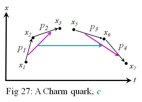
There are two spatial jumps on each side of the aqua arrow in both Fig 25 and Fig 26. Each jump generally occurs at different times in Fig 25. But there are sequences of jumps on each side in Fig 26. So it represents changes in direction and more energy associated with those changes in direction. Fig 26 still represents a quark since the strong arrow is the only arrow left exposed in the middle and available for connection by a gluon. It has the same charge as an Up quark, but now has more energy/mass. So I call it a Charm quark, c. And it has its anti-matter partner, the Anti-Charm quark, c̅.
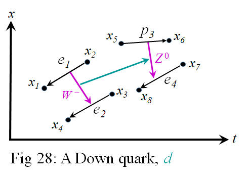
We can also start with a down quark as shown in Fig 28.
If we let x4 = x2, and x6 = x7, then we get the particle configuration of Fig 29.
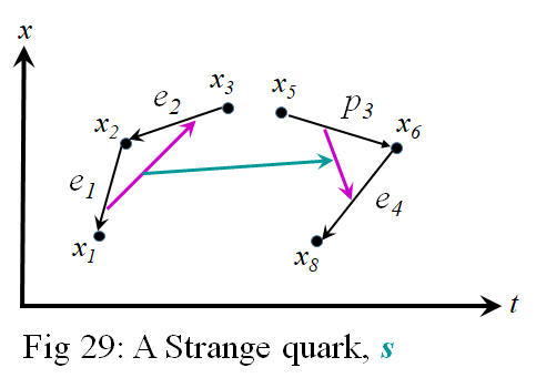
Here again we have a series of spacetime jumps on each side of the strong arrow which represent more energy associated with changing direction. So it has the same electric charge as the down quark, but has more energy. I call it a Strange quark, s. And it has its anti-particle partner, the Anti-strange quark, s̅.
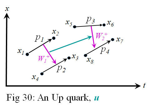
Or start again with an Up quark, shown again in Fig 30.
If we connect x2 to x4 with a p and connect x6 to x8 with another p, we get the configuration of Fig 31.
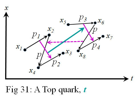
With these added positrons, we now have a series of 3 spacetime jumps on each side of the strong arrow. And so this particle has more energy than the previous c quark. I would call it a Top quark, t. Although the magenta arrows intersect the newly added p arrows, they are not connected to them. However, the new p arrows might be connected by the dashed magenta arrow. All these added connections and shared nodes seem like it might be more difficult to construct and maintain and are probably more unstable. I expect they would break apart relatively quickly.
And if we start with a down quark as shown again in Fig 32,
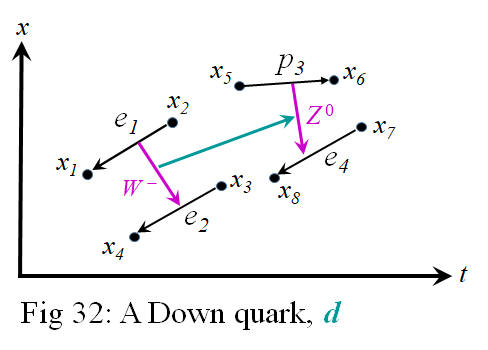
we can connect x4 to x2 with a p and connect x6 to x7 with a p (or perhaps an e). This would give us the configuration of Fig 33.

And we get a particle with the same charge as the down quark but with more energy than the strange quark. So I call it a Bottom quark, b. Its antiparticle partner is the Anti-bottom quark, b̅.
Just out of curiosity, I wonder if there is a particle with the configuration of Fig 34.
This particle is achieved by using the tau particle in Fig 26 and connecting x1 to x7. It would be electrically neutral. And it seems its strong and weak arrows are shielded from making connections by the electrical charges. So it might not interact with known matter particles. Could this be a dark matter particle?
But what might neutrinos be? Neutrinos have almost no mass, they rarely interact with other particles, and they only interact through the weak force. This means that neutrinos are the result of the decay of and bosons. For example, a particle will decay into an electron and a neutrino. Let's draw these configurations to see how a neutrino might be configured. See Fig 35.
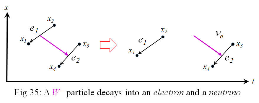
Here, a
particle on the left decays into an electron, e1, and a neutrino,
, on the
right. But we have an electric charge on the left of
, and what seems to be a
charge of
on the
left with e1 and e2. So
we must remedy this if we wish to maintain consistency of charge on both
sides. We can fix this if we let
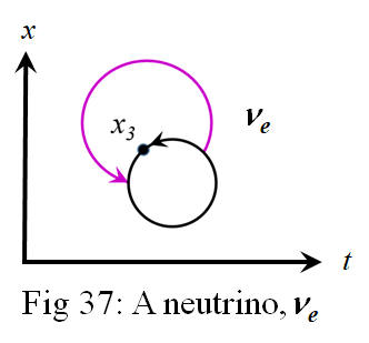
If we can connect the head of one arrow to the tail of another to create a muon as was done in Fig 23, then it should be just as easy to connect the head of one arrow to its own tail as shown in Fig 36. And since this circle has just as much of the line going forward as backwards in time, it has a net zero electric charge. Now we have a charge of on both sides of Fig 35, and we have an electrically neutral neutrino just as the Standard Model does. Also, since the black arrow ends at the same place it started, there is no information nor energy propagated to a different point in space. But perhaps there is energy transmitted through the magenta arrow.
However, we still have the tail of the magenta weak arrow floating without a connection in Fig 36. We can't have this because any arrow here represents a subtraction of two quantities. A floating tail represents a subtraction of nothing when both sides of the minus side are required. Since the quantities on both sides of the subtraction can be commuted to form the anti-particle, both have equal status, and you cannot go without one or the other.
If the black, electric arrow can end at the same point where it began, then the magenta weak arrow can end on the same black arrow where it began. See Fig 37.
Since space is 3D, having the magenta arrow outside the black arrow is equivalent, topologically, to having the magenta arrow inside the black arrow, as shown in Fig 38.
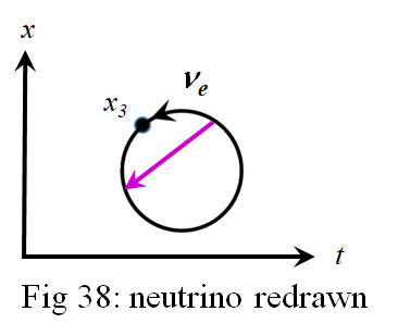
Now it can be seen that the magenta arrow is pulling together the black arrow so it ends where it began.
But the question is how would such a particle propagate through the spacetime points. If the black arrow can close in on itself, then it can open up to start on a different point than where it began. Then it can close on this different point. It would open and close on different points along a path and in this way propagate from point to point. Perhaps a shorter magenta arrow represents less energy, and perhaps the length of this arrow oscillates, causing the black arrow to seek different starting or ending points.
We also have that the muon decays into a particle and a neutrino. If we draw this interaction in terms of the framework here, we get Fig 39.
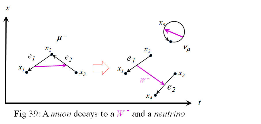
It seems a neutrino spontaneously
forms at
And we might wonder if a neutrino could break any bond of electrons or positrons? For example, could a neutrino break apart or pull together the electrons on only one side of the strong arrow in an anti-charm or anti-top quark? If it did, then the quark that would result would be unbalanced and would probably not hold together. There would be more energy on one side of the strong arrow than on the other, and would fly apart. Or perhaps such particles do exist for the briefest of moments such that we haven't seen them yet. If we have a wave function for composite particles such as these, the math would probably show which combinations are stable, why, and how fast unstable versions would last.
And finally, there is the photon. Photons have no rest mass or charge and always travel at the speed of light. They are created by particle/anti-particle collisions, they annihilate by creating particle/anti-particle pair production, and they interact with electrically charged particles. So photons interact with electrons, muons, and tau particles and their anti-particles, photons interact with quarks and anti-quarks, and photons interact with the W bosons. But photons do not interact with neutrinos, the Z bosons, or gluons, since these don't have a net electric charge.
The question then, is how are photons represented in terms of this framework. Are photons an elementary particle with no constituents, or are they a composite particle like many described so far? If a photon is created out of the debris of particle/anti-particle collisions, or if a particle/anti-particles can combine to form a photon, this suggest that a photon is a composite of at least an electron and a positron. But how could the combination of two particles with mass form a particle with no mass?
If we have both an electron and a positron traveling together from x1 to x2 in time t1 to t2, then we have in essence two alternative paths from x1 to x2. This puts the electron and positron in superposition and their individual transition amplitudes get added to form the wave function of the photon they create. So to create a photon, we add the positron amplitude of Equation [34] to the electron amplitude of Equation [35], to get,
.
And the second term can be manipulated to get,
. Which is equal to,
.
.
But when multiplying exponentials of the same number, e, we can add the
exponents to get,
.
Then we can take the imaginary number in the denominator of the square-root and modified
it to
, and we get,
.
The
can be added to each exponent to get,
. Now the sum of exponentials is of the form,
,
with
.
So finally this gives us a photon amplitude of,
.
We can recognize that,
,
which is equal to,
.
Notice that E has the units of Joules, [J],
has the units of seconds, [s], and
has the units of Joule-seconds, [Js]. So
has the units of
[J][s]/[Js]=1, which mean that expression is dimensionless, it has no units. And
this is what is require for it to be the argument of the cosine function. The
argument of a sine or cosine function is an angle which has no units of measure.
Yet the cosine function is typical of a wave travelling through space and time.
We have the time portion,
, so can we express the energy, E, in terms of a variable more
related to a wave, such as frequency? If we let
,
where is the angular frequency, then
again the argument of the cosine is dimensionless, as required. The equation,
, is known as the Planck-Einstein relation for the energy of a photon. And so our cosine function starts at
x1 at t1
with the phase angle,
, and it end at x2 at t2, with the
phase angel,
. Interactions So far the framework of quantum theory has been derived
here
from first principles. And the implications and higher implications have been
correlated to particles. All this seems to match the Standard Model. But these
considerations will be more credible if the various interactions of the Standard
Model can be explained in terms of this framework. How exactly do the particles
here interact? I've shown how the
and the muon decay resulting in other particles and neutrinos. But there are quite a
few more interactions to explain. Fig 40 shows what types of particles interact
with which other types of particles. For example, the gluon only interact with
themselves and the quarks. The neutrino interactions always involve a
or
boson. The leptons do not directly interact with the quarks. And photons
do not interact with the neutrinos, the gluon, the
boson, nor other photons. All these interactions and lack of interactions need
to be explained with this framework.
Individual interactions are usually depicted with Feynman diagrams, where a
particle is depicted as a straight, wavy, or curly line, depending on the type
of particle. In a Feynman diagram a particle or particles are shown to come in
on the left, meet in the middle at a vertex (a dot), and other combinations of
particles are shown to leave at the right. For example, the Feynman diagram of
the
decaying to an electron and a neutrino is
shown in Fig 41
below.
Section
8
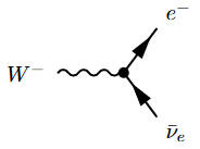
Fig 41:
The more complete list of Feynman diagrams with one vertex is shown here. Keep in mind that you can rotate Fig 41 so that any others of those particles are coming in. So, for example, we can rotate Fig 41 so that the electron and neutrino are coming in and the Weak boson is going out as shown in Fig 42.
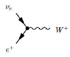
Fig 42:
e+ +
But now, with time increasing from left to right on the page, the , electron, and neutrino are going in the reverse direction in time. This makes the Weak boson a particle, the electron converts to a positron, and the neutrino converts to its anti-particle. Yet this is still a valid interaction.
In the Standard Model there is no explanation given for why these interactions are permissible. But if the framework here has merit, then it may give a reason for these particular interactions; it may explain what's happening inside the vertices.
The first interaction to consider is the photon with the electron. Fig 43 shows a photon consisting of e1 and p2 coming in from the left and encountering an electron, e2.
The positron part of the photon establishes a connection with e2 to become a different photon than before. Since e2 does not have an opposite phase angle as p2, they do not cancel each other out but form a separate photon instead. The new photon consisting of p2 and e2 continues in a different direction. This leaves the electron, e1, floating off by itself. Since all electrons look the same, this interaction appears to be a photon bouncing off the an electron and imparting some momentum to it.
conservation of charge connections
Interactions, decays, superposition of all possible interaction to create the field version of the path integral, and how it relates to Feynman diagrams.
coupling constants
Conclusion
In the Standard Model, there is assigned a separate mathematical field for each type of particle, a field for the electrons and positrons, a field for the quarks and anti-quarks, a field for the photons, a field for gluons, and a field for the neutrinos, etc. Each type of particle is considered elemental; there is no common substructure to explain them. When particles are capable of influencing each other by interacting, the strength of the interaction is determined by a coupling constant. All the various coupling constants are determined by experimental data. The existence of all the particles and how they interact is determined from direct and indirect observational data alone. There is no fundamental principles to derive quantum theory or the particles to which it applies. The math used is only used because it fits the data from experiment.
Here, however, is described a common substructure from which all the various particles are produced. The reason that this substructure in not discernible by modern methods is that each type of particle is constructed of differentials in the path integral. So each type of particle is again its own differential in a path integral. And as such, differential quantities in an integral are not directly observable, only their accumulative effects can be calculated and observed.
![]()